Download
1 / 52
520 likes | 622 Views
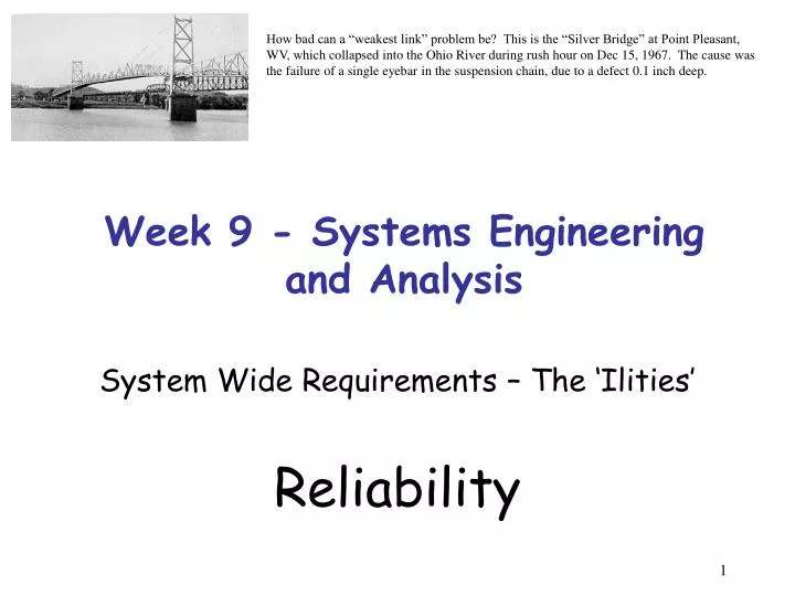
How bad can a “weakest link” problem be? This is the “Silver Bridge” at Point Pleasant, WV, which collapsed into the Ohio River during rush hour on Dec 15, 1967. The cause was the failure of a single eyebar in the suspension chain, due to a defect 0.1 inch deep.

E N D
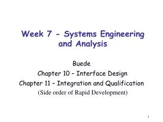
How bad can a “weakest link” problem be? This is the “Silver Bridge” at Point Pleasant, WV, which collapsed into the Ohio River during rush hour on Dec 15, 1967. The cause was the failure of a single eyebar in the suspension chain, due to a defect 0.1 inch deep. Week 9 - Systems Engineering and Analysis System Wide Requirements – The ‘Ilities’ Reliability
Engineering disasters… AT&T network map AT&T Network Crash story (last week’s links) Kansas City Hotel story (ditto) Challenger (tonight’s slides)
The Ilities • Quality • Reliability – • Blanchard and Fabrycky – Ch 12 • Wasson – Ch 50 • Interoperability • Usability • Maintainability • Serviceability • Producibility and Disposability
The Ilities-2 • All are System Wide in Scope. • All are desirable system outcomes. • Technical, engineering, mathematical definitions behind each one. • Included as Technology and System-Wide requirements when critical enough. • How to measure and quantify ?
The Second ‘Ility’ - Reliability • Our focus – • Reliability Definitions. • Series and Parallel Systems. • Reliability Improvement Methods. • Reliability Prediction and Testing. • Risk (Ch. 19)
Definition of Reliability • The reliability of an item is the probability that it will adequately perform its function for a specified period of time. • ‘Time’ is involved • specify units – hrs, miles, etc. • specify time duration.
Reliability vs. Quality • Reliability : includes passage of time. • Quality : static descriptor. • High reliability implies high quality – converse not true. • Tire example – • Ones made in 1960 and 2000. • Both ‘high quality’ wrt current standards • New ones last longer – more reliable.
Reliability Example • Space Shuttle Challenger accident on January 28, 1986. • O-Rings sealed the joints in the solid rocket motors. • Engineers used two O-rings – one for ‘backup’. • Launch ‘reliability’ calculated as 0.87 at 31 deg F. (0.98 at 60 deg F).
Launch Details • During flight, the rocket casing ‘bulges’ which widens the gap between sections. • Due to low temperature and bulging effect – both O-rings failed resulting in accident. (not independent systems). • Launch ‘reliability’ calculated as 0.87 at 31 deg F. (0.98 at 60 deg F).
Three Aspects of Reliability • Analysis – how to quantify, equations • Testing – how to test • Prediction – how do I know in advance
Measures of Reliability (12.2) • Reliability Function, R(t) – probability that system will be successful for some time period t. • R(t) = 1 – F(t) • F(t) is the failure distribution or ‘unreliability’ function.
R(t) for Exponential distn. Integral from t to infinity is “the rest of the probability” beyond t, i.e., the probability it didn’t fail up to time t. • R(t) = 1 – F(t) = • If ‘time to failure’ is (assumed to be) defined by Exponential Function (Constant Failure Rate) then – f(t) =
Resulting R(t) function • R(t) = • Mean life (q) is average lifetime of all items considered. • For exponential distribution, MTBF is q.
Failure rate and MTBF • R(t) = = • l is instantaneous failure rate • M or q are MTBF. • l = 1/q = 1/MTBF
Wasson MTTF Light bulb failures
Wasson MTBF • Wasson suggests • MTBF = MTTF + MTTR • Mean Time Between Failures • Mean Time To Failure • Mean Time To Repair • Since MTTR is small, MTBF approx = MTTF
The Failure Rate • Failure Rate is: • Number of Failures/Total Operating Hrs • Failure rate expressed as failures per hour, failures per million hours, etc.
Failure Rate Example • 10 Components tested for 600 hrs. • Failure Rate per hr, l = 5/4180 = 0.001196 • MTBF= ??
Reliability Nomograph - Fig 12.3 • For exponential distribution. • Relationship between MTBF, l, R(t). • Example : MTBF is 200 hrs (l=0.005) and operating time is 2 hrs – then R(t) =0.99
Wasson – Bathtub Curve ‘Burn-in’ of electronics devices
Reliability of Component Relationships • Engineers assemble systems from components and sub-systems. • How to analyze the reliability of the ‘whole’ based on structure and component reliabilities. • Two simple structures : series and parallel.
Series Networks • Series components – all must function. • R = (RA ) (RB ) (RC) (multiply R’s) • R = (add l’s)
Sample Problem – Series • Series system of four components, expected to operate to 1000 hrs. • MTBFs – • A (6000 hrs), B(4500), C(10500), D(3200) • What is R for the series system ?? • (Ans. 0.4507) • What is MTBF for the series system ??
Parallel Networks • Parallel components – all must fail for system to fail. • R = RA + RB – (RARB) • R = 1 – (1 – RA) (1 – RB) (1 – RC)… • (n components)
Series and Parallel Networks • Figure 12.10- Reduce parallel blocks to equivalent series element.
Sample Problems • Figure 12.10 ‘a’ and ‘c’. • RA = 0.99 • RB = 0.96 • RC = 0.98 • RD = 0.92 • RE = 0.8 • RF = 0.8
Related Figures of Merit (FOM) • Mean Time Between Maintenance – MTBM • Scheduled • Unscheduled • Availability – A • Probability that system when used under stated conditions in ‘ideal/actual’ operational environment will operate satisfactorily. • Wasson – RAM • Reliability • Availability • Maintenance
Figure 12.11 • How to calculate MTBF, MTBM ?? • MTBF – 58 failed ? • MTBM – 100 ‘failed’ ? A Common Service Shop Finding – NTF, no trouble found
Reliability and System Life Cycles – section 12.3 • What Reliability should the System have to accomplish mission, over life cycle, under expected environment. • Requirements that affect reliability • System performance factors, • Mission profile, • Use conditions, duty cycle, etc. • Environment – temp, vibration, etc.
Review of Key Concepts • ‘Ilities’ are System Wide Requirements. • Specify ‘Reliability’ as MTBF, MTBM, R(t),.. • Flow down/allocate top level requirements to functional blocks (Fig 12.16,17) • We have functional architecture. • We have series/parallel tools to do this.
Reliability Flow Down Series : Add lambdas Series : Add lambdas MTBFs have to get larger - See slide 33
Reliability Prediction • Predict based on similar equipment – easy but inaccurate. • Predict from Parts Count • Predict from Life/Stress Analysis
Example – Parts Count where: n = Number of part categories Ni = Quantity of ith part λ= Failure rate of ith part π= Quality Factor of ith part(handbook)
MTBF = 1/l where: n = Number of part categories Ni = Quantity of ith part λ= Failure rate of ith part π= Quality Factor of ith part(handbook)
Reliability Testing - 12.6 • Part of test and qualification. • Assure that MTBF requirements are met. • Testing : • Either accept, reject, continue test (Fig. 12.30) • Test under simulated mission profile (Fig 12.31) ‘Run some tests’ – how confident are we in the results ??
Reliability Testing-2 • Establish criteria for accept, reject, and risks of false decisions. • Equations 12.29, 12.30. Determine regions for accept, reject, continue, with defined acceptance risks.