Download
1 / 44
440 likes | 555 Views
Geomagnetic Indices Regular Irregularity and Irregular Regularity A Journey. Leif Svalgaard Stanford University leif@leif.org IAGA 11 th 2009 H02-FRI-O1430-550 (Invited). Regular Variations.

E N D
Geomagnetic IndicesRegular Irregularity and Irregular RegularityA Journey Leif Svalgaard Stanford University leif@leif.org IAGA 11th 2009 H02-FRI-O1430-550 (Invited)
Regular Variations George Graham discovered [1722] that the geomagnetic field varied during the day in a regular manner. He also noted that the variations were larger on some days than on other days. So even the ‘regular’ was irregular…
Disturbances and Aurorae Pehr Wargentin [1750] also noted the regular diurnal variation, but found that the variation was ‘disturbed’ at times of occurrence of Aurorae. Graham, Anders Celsius, and Olaf Hjorter had earlier also observed this remarkable relationship.
The First Index (Regular–Irregular) John Canton [1759] made ~4000 observations of the Declination on 603 days and noted that 574 of these days showed a ‘regular’ variation, while the remainder (on which aurorae were ‘always’ seen) had an ‘irregular’ diurnal variation.
Classification - Character The First Index was thus a classification based on the ‘character’ of the variation, with less regard for its amplitude, and the ancestor of the C-index (0=quiet, 1=ordinary, 2=disturbed) that is still being derived today at many stations. The availability of the Character Index enabled Canton to discover another Regularity on Quiet days.
More than One Cause And to conclude that “The irregular diurnal variation must arise from some other cause than that of heat communicated by the sun” This was also evident from the association of days of irregular variation with the presence of aurorae
Another Regular Variation George Gilpin [1806] urged that regular measurements should be taken at fixed times during the day. And demonstrated that the seasonal variation itself varied in a regular manner George Gilpin sailed on the Resolution during Cook's second voyage as assistant to William Wales, the astronomer. He joined on 29 May 1772 as astronomer's servant. John Elliott described Gilpin as "a quiet yg. Man". Gilpin was elected Clerk and Housekeeper for the Royal Society of London on 03 March 1785 and remained in these positions until his death in 1810.
Hint of Sunspot Cycle Variationthough unknown to Gilpin, who thought he saw a temperature effect
Alas, Paradise Lost Canton’s great insight [that there were different causes of the variations during quiet and disturbed times] was lost with Gilpin and some later workers, and a new and simpler ‘index’ won acceptance, namely that of the Daily Range. The ‘raw’ Daily Range is, however, a mixture of effects.
The Daily Range Index The Daily Range is simple to calculate and is an ‘objective’ measure. It was eventually noted [Wolf, 1854] that the range in the Declination is a proxy for the Sunspot Number defined by him.
Rudolf Wolf’s Sunspot Number Wolf used this correlation to calibrate the sunspot counts by other observers that did not overlap in time with himself
How to Measure Disturbance Edward Sabine [1843], mindful of Canton’s insight, computed the hourly mean values for each month, omitting ‘the most disturbed days’ and defined Disturbance as the RMS of the differences between the actual and mean values.
The Ever-present Tension • Quiet time variations – their regular and irregular aspects • Disturbance variations – their irregular and regular aspects One cannot conclude that every regularity is a sign of ‘quiet’ and that every irregularity is a sign of ‘activity’. This is an important lesson.
Quiet Time Variations • Diurnal 25 nT • Focus Change of sign (irregular) • Lunar Phase X 0.1 • Annual X 2 • Solar Cycle X 3 (irregular) • Secular 10%/century (irregular) Mixture of regular and irregular changes
Disturbance Variations • Sporadic Storms 300 nT • Recurrent Storms 100 nT (recurrent) • Semiannual/UT var. 25% (modulation) • Annual 5% (modulation) • Bays 20-50 nT • Secular ? Mixture of irregular and regular changes Note: As seen at mid-latitudes
Qualitative Indices An index can be a short-hand code that captures an essential quality of a complex phenomenon, e.g. the C-index or the K-index:
Quantitative Indices We also use the word index as meaning a quantitative measure as a function of time of a physical aspect of the phenomenon, e.g. the Dst-index or the lesser known Tromsø Storminess-index:
Model of Geomagnetic Variations It is customary to decompose the observed variations of the field B, e.g. for a given station to first order at time t: B (t) = Bo(t) + Q(l,d,t) + D(t)∙M(u,d) where u is UT, d is day of year, l is local time, and M is a modulation factor. To second order it becomes a lot more complex which we shall ignore here.
Separation of Causes To define an index expressing the effect of a physical cause is now a question of subtraction, e.g.: D(t)∙M(u,d) = B (t) – [Bo(t) + Q(l,d,t)] or even D(t)= {B (t) – [Bo(t) + Q(l,d,t)]} / M(u,d) where M can be set equal to 1, to include the modulation, or else extracted from a conversion table to remove the modulation
Fundamental Contributions Julius Bartels [1939,1949] • Remove Bo and Q judiciously, no ‘iron curve’ • Timescale 3 hours, match typical duration • Scale to match station, defined by limit for K = 9 • Quasi-logarithmic scale, define a typical class to match precision with activity level
The Expert Observer Pierre-Noël Mayaud, SJ [1967;1972] put Bartels’ ideas to full use with the am and aa-indices. A subtle, very important difference with Bartels’ Ap is that the modulation, M, is not removed and thus can be studied in its own right.
Exists both for Southwards and for Northward fields (permanent feature)
Relative Magnitude Independent of Sign of Bz (Varies 30% or more)
(1 + 3 cos2(Ψ)) is Basically Variation of Field Strength Around a Dipole
The Lesson From Mayaud • Mayaud stressed again and again not to use the ‘iron curve’, and pointed out that the observer should have a repertoire of ‘possible’ magnetogram curves for his station, and ‘if in doubt, proceed quickly’. • He taught many observers how to do this. Unfortunately that knowledge is now lost with the passing of time [and of people].
Since Determination of the Quiet Field During Day Hours is so Difficult, We Decided to Only Use Data Within ±3 Three Hours of Midnight (The IHV Index)
The Midnight Data Shows the Very Same Semiannual/UT Modulation as all Other Geomagnetic Indices (The ‘Hourglass’)
The Many Stations Used for IHVin 14 ‘Boxes’ well Distributed in Longitude, Plus Equatorial Belt
IHV is a Measure of Power Input to the Ionosphere (Measured by POES)
IHV has Very Strong (Slightly Non-Linear) Relation with Am-index
We can also Determine BV2 Solar Wind Coupling Function Am ~ BV2
Bartels’ u-measure and our IDV- index u: all day |diff|, 1 day apart IDV: midnight hour |diff|, 1 day apart
IDV is Blind to V, but has a Significant Relationship with HMF B The HMF back to 1900 is strongly constrained
We Can Even [With Less Confidence] Go Back to the 1830s From IHV-index we get BV2 = f(IHV) From IDV-index we get B = g(IDV) From PC-index we get BV = h(PCI) Which is an over-determined system allowing B and V to be found and cross-checked
Conclusion • From Canton, Sabine, Wolf, Bartels, and Mayaud, the patient recording [by many people] and growing physical insight have brought us to heights that they hardly could have imagined, but certainly would have delighted in. From their shoulders we see far. “Ban the iron curve, whether wielded by human or by machine” The End
Abstract Geomagnetic variation is an extremely complicated phenomenon with multiple causes operating on many time scales, characterized by 'regular irregularity, and irregular regularity'. The immense complexity of geomagnetic variations becomes tractable by the introduction of suitable geomagnetic indices on a variety of time scales, some specifically targeting particular mechanisms and physical causes. We review the historical evolution of the 'art of devising indices'. Different indices [by design] respond to different combinations of solar wind and solar activity parameters and in Bartels' [1932] words "yield supplemental independent information about solar conditions" and , in fact, have allowed us to derive quantitative determination of solar wind parameters over the past 170 years. Geomagnetic indices are even more important today as they are used as input to forecasting of space weather and terrestrial responses.