Download
1 / 45
450 likes | 615 Views
The Seasonal Forecast System at ECMWF. Tim Stockdale European Centre for Medium-Range Weather Forecasts. Contents. Seasonal forecasting with coupled GCMs Why use GCMs? How we make a forecast Basic calibration – how, why, and what are the problems? Model error

E N D
The Seasonal Forecast System at ECMWF Tim Stockdale European Centre for Medium-Range Weather Forecasts
Contents • Seasonal forecasting with coupled GCMs • Why use GCMs? • How we make a forecast • Basic calibration – how, why, and what are the problems? • Model error • Operational forecasts: ECMWF System 4 • System design • How good are the El Nino forecasts? • How good are the atmospheric forecasts? • Forecast interpretation • Meaning of probabilistic forecasts • Outlook
Sources of seasonal predictability • KNOWN TO BE IMPORTANT: • El Nino variability - biggest single signal • Other tropical ocean SST - important, but multifarious • Climate change - especially important in mid-latitudes • Local land surface conditions - e.g. soil moisture in spring • OTHER FACTORS: • Volcanic eruptions - definitely important for large events • Mid-latitude ocean temperatures - still somewhat controversial • Remote soil moisture/ snow cover - not well established • Sea ice anomalies - local effects, but remote? • Dynamic memory of atmosphere - most likely on 1-2 months • Stratospheric influences - solar cycle, QBO, ozone, … • Unknown or Unexpected - ???
Methods of seasonal forecasting • Empirical forecasting • Use past observational record and statistical methods • Works with reality instead of error-prone numerical models • Limited number of past cases means that it works best when observed variability is dominated by a single source of predictability • A non-stationary climate is problematic • Two-tier forecast systems • First predict SST anomalies (ENSO or global; dynamical or statistical) • Use ensemble of atmosphere GCMs to predict global response • Many people still use regression of a predicted El Nino index on a local variable of interest • Single-tier GCM forecasts • Include comprehensive range of sources of predictability • Predict joint evolution of SST and atmosphere flow • Includes indeterminacy of future SST, important for prob. forecasts • Model errors are an issue!
Step 1: Build a coupled model • IFS (atmosphere) • TL255L91 Cy36r4, 0.7 deg grid for physics (operational in Nov 2010) • Modifications to stratospheric physics and lakes • Singular vectors from EPS system to perturb atmosphere initial conditions • Ocean currents coupled to atmosphere boundary layer calculations • NEMO (ocean) • Global ocean model, 1x1 mid-latitude resolution, 0.3 near equator • Sophisticated 3D-VAR ocean analysis system, including analysis of salinity, multivariate bias corrections and use of altimetry. • Coupling • Fully coupled, no flux adjustments, except no physical model of sea-ice
Step 2: Make some forecasts • Initialize coupled system (cf Magdalena’s lecture) • Aim is to start system close to reality. Accurate SST is particularly important, plus ocean sub-surface. • Don’t worry too much about “imbalances” • Run an ensemble forecast • Explicitly generate an ensemble on the 1st of each month, with perturbations to represent the uncertainty in the initial conditions; run forecasts for 7 months • Worry about model error later ….
Creating the ensemble • Wind perturbations • Perfect wind would give a good ocean analysis, but uncertainties are significant. We represent these by adding perturbations to the wind used in the ocean analysis system. • BUT only have 5 member ensemble, and only limited representation of other sources of uncertainty in ocean analysis (e.g. obs error) • SST perturbations • SST uncertainty is not negligible • SST perturbations added to each ensemble member at start of forecast. • BUT perturbations based on SST analyses that used the same input data • Atmospheric unpredictability • Atmospheric ‘noise’ soon becomes the dominant source of spread in an ensemble forecast. This sets a fundamental limit to forecast quality. • To ensure that noise grows rapidly enough in the first few days, we activate ‘stochastic physics’ and use EPS singular vectors. • In System 4, stochastic physics increases spread at all timescales.
.. but ensemble spread (dashed lines) is still substantially less than actual forecast error. Substantial amounts of forecast error are not from the initial conditions. RMSE and spread in different systems Rms error of forecasts has been systematically reduced (solid lines) ….
Step 3: Remove systematic errors • Model drift is typically comparable to signal • Both SST and atmosphere fields • Forecasts are made relative to past model integrations • Model climate estimated from 30 years of forecasts (1981-2010), all of which use a 15 member ensemble. Thus the climate has 450 members. • Model climate has both a mean and a distribution, allowing us to estimate e.g. tercile boundaries. • Model climate is a function of start date and forecast lead time. • EXCEPTION: Nino SST indices are bias corrected to absolute values, and anomalies are displayed w.r.t. a 1971-2000 climate. • Implicit assumption of linearity • We implicitly assume that a shift in the model forecast relative to the model climate corresponds to the expected shift in a true forecast relative to the true climate, despite differences between model and true climate. • Most of the time, assumption seems to work pretty well. But not always.
Biases (eg JJA 2mT as shown here) are often comparable in magnitude to the anomalies which we seek to predict ECMWF Met Office Météo-France CFS Plots courtesy Paco Doblas-Reyes
SST bias is a function of lead time and season. Some systems have less bias, but it is still large enough to require correcting for.
Nino plumes: variance scaling • Model Nino SST anomalies in S4 have too large amplitude • Problem is especially acute in boreal spring and early summer (model bias of “permanent La Nina” does not allow spring relaxation physics to apply; this was something S3 did very well) • We plot the “Nino plumes” corrected for both mean and variance, instead of just the mean. • This is done by scaling the model anomalies so that the model variance matches the observed variance in the calibration period • We use the same approach (cross-validated) when calculating scores • This affects the plotting, not the model data itself • The spatial maps are not affected: the tercile and quintile probability maps are already implicitly standardized wrt model variance • General technique: is also used in our multi-model system
Variance adjusted Unadjusted model anomalies
Despite SST bias and other errors, anomalies in the coupled system can be remarkably similar to those obtained using observed (unbiased) SSTs …..
Model errors are still serious … • Models have errors other than mean bias • Eg weak wind and SST variability in System 2 • Past models underestimated MJO activity (S4 better) • Suspected too-weak teleconnections to mid-latitudes • Mean state errors interact with model variability • Nino 4 region is very sensitive (cold tongue/warm pool boundary) • Atlantic variability suppressed if mean state is badly wrong • Forecast errors are often larger than they should be • With respect to internal variability estimates and (occasionally) other prediction systems • Reliability of probabilistic forecasts is often not particularly high (S4 better)
Capturing trends is important. Time-varying CO2 and other factors are important in this. There is a strong link between seasonal prediction and decadal/ multi-decadal climate prediction.
Operational seasonal forecasts • Real time forecasts since 1997 • “System 1” initially made public as “experimental” in Dec 1997 • System 2 started running in August 2001, released in early 2002 • System 3 started running in Sept 2006, operational in March 2007 • System 4 started running in July 2011, operational in November 2011 • Burst mode ensemble forecast • Initial conditions are valid for 0Z on the 1st of a month • Forecasts are usually complete by late on the 2nd. • Forecast and product release date is 12Z on the 8th. • Range of operational products • Moderately extensive set of graphical products on web • Raw data in MARS • Formal dissemination of real time forecast data
System 4 configuration • Real time forecasts: • 51 member ensemble forecast to 7 months • SST and atmos. perturbations added to each member • 15 member ensemble forecast to 13 months • Designed to give an ‘outlook’ for ENSO • Only once per quarter (Feb, May, Aug and Nov starts) • Back integrations from 1981-2010 (30 years) • 15 member ensemble every month • 15 members extended to 13 months once per quarter
How many back integrations? • Back integrations dominate total cost of system • System 4:5400 back integrations (must be in first year) • 612 real-time integrations (per year) • Back integrations define model climate • Need both climate mean and the pdf, latter needs large sample • May prefer to use a “recent” period (30 years? Or less??) • System 2 had a 75 member “climate”, S3 had 275, S4 has 450. • Sampling is basically OK • Back integrations provide information on skill • A forecast cannot be used unless we know (or assume) its level of skill • Observations have only 1 member, so large ensembles are less helpful than large numbers of cases. • Care needed e.g. to estimate skill of 51 member ensemble based on past performance of 15 member ensemble • For regions of high signal/noise, System 4 gives adequate skill estimates • For regions of low signal/noise (eg <= 0.5), need hundreds of years
Land surface Snow depth limits, 1st April
QBO System 4 30hPa System 3 50hPa
Ozone S4 uses interactive ozone, which is able to improve temperature forecasts in the stratosphere. Ozone re-analyses are dominated by spurious changes, and cannot be used to initialize forecasts. For S4, we were forced to use a climatological initial condition instead.
Stratospheric trends Stratospheric temperature trend problem. This is due to an erroneous trend in initial conditions of stratospheric water vapour.
Example forecast products • A few examples only – see web pages for full details and assessment of skill • All graphical products come with corresponding skill estimate • Note: Significance values on plots • A lot of variability in seasonal mean values is due to chaos • Ensembles are large enough to test whether any apparent signals are real shifts in the model pdf • We use the w-test, non-parametric, based on the rank distribution • NOT related to past levels of skill
ENSO Past performance
SST forecast performance Actual rms errors > model estimate of “perfect model” errors
More recent SST forecasts are better .... 1996-2010 1981-1995
How good are the forecasts? Deterministic skill: DJF ACC Perfect model estimate (S3) Actual forecasts (S3) T2m Precip
S4 prediction skill Note: estimated here from 51 member ensemble
How good are the forecasts? Probabilistic skill: Reliability diagrams Tropical precip < lower tercile, JJA Global T850 > upper tercile, DJF
How good are the forecasts? Probabilistic skill: Reliability diagrams Europe: Temp > upper tercile, JJA and DJF
Model error and forecast interpretation • Model error is large • It still dominates some SST forecast errors (e.g. west Pacific) • Mean state and variability errors are very significant • Errors cannot be easily fixed • Products typically account for sampling error only • Don’t take model probabilities as true probabilities • Estimating forecast skill can be difficult • In many cases, data is insufficient to produce sensible estimates • This problem will not go away • In the end we need trustworthy models • (Multi-model ensembles are small, and only partially span the space of model errors)
Calibrated forecasts • Frequentist or Bayesian • Sampling uncertainties give rise to frequentist probabilities • Model errors mean our forecast pdfs are wrong. We can try to represent our lack of knowledge as “probabilities” in a Bayesian framework. • Calibration of probabilistic forecasts • Given the model forecast pdf, the past history of forecast pdfs, the past history of observed outcomes, what is the best estimate of the true pdf? • A Bayesian analysis depends on specification of the prior. Mathematically, no single “right” answer. • We hope one day to implement a hierarchical Bayesian analysis, accounting for the major uncertainties and producing some general purpose calibrated probabilistic forecasts. • Handling trends and non-stationarities is an additional challenge
Some final comments • Plenty of scope for improving model forecasts • Nino SST forecasts still significantly worse than predictability limits • Model errors still obvious in many cases, some processes poorly treated • Ocean initial conditions probably OK in Pacific for reasonable number of years, recently improved elsewhere by ARGO • Model output -> use of forecast • Calibration and presentation of forecast information • Potential for multi-model ensembles • Integration with decision making • Timescale for improvements • Optimist: in 10 years, we’ll have much better models, pretty reliable forecasts, confidence in our ability to handle climate variations • Pessimist: in 10 years, modelling will still be a hard problem, and progress will largely be down to improved calibration