Download
1 / 48
600 likes | 994 Views
Modeling Repeated Measures or Longitudinal Data. Example: Annual Assessment of Renal Function in Hypertensive Patients. responses for each subject are vectors. typical for some time points to be missed. Example: Annual Assessment of Renal Function in Hypertensive Patients.

E N D
Example: Annual Assessment of Renal Function in Hypertensive Patients responses for each subject are vectors typical for some time points to be missed
Example: Annual Assessment of Renal Function in Hypertensive Patients • May want to examine: • Change in renal function over time • Effect of covariates on renal function • Interactions between covariates and time (i.e. do covariate effects differ over time) Mean EGFR by Year Analysis must account for the correlation between observations taken from the same subject.
Are the observations correlated in our renal function example? Correlation Matrix for EGFR
Example: Annual Assessment of Renal Function in Hypertensive Patients • Other issues: • Sample size is not constant (“unbalanced design”) • How should time be modeled? • Are missing data and/or censoring a problem?
Repeated Measures ANCOVA Typically used for responses collected at similar time points Repeated measures models do not distinguish between sources of variation treat within-subject covariance as “nuisance” use structured covariance matrices and weighted least-squares Model interests are mean response profiles and relationships with covariates:
General Linear Mixed Model • Recall the “GLM”: • Extension of General Linear Model: There is only one source of random variation in the above equation, assuming fixed effects • Whenever a factor is considered to be random, it is a sample from a distribution of levels, and now the factor or variable brings a new source of random variation to the model • The general linear mixed model is the most flexible approach for incorporating random effects
TIME OUT: matrix notation • Matrix: a 2-dimensional array of numbers • Typical design matrix for the i-th subject with p covariates and k assessments: • If β is a p×1 vector, then Xi•βis
General Linear Mixed Model • Xi is the usual design matrix of fixed effects for the i-th • βis a vector (i.e., a k×1 matrix) of regression coefficients • Zi is a design matrix of random effects for the i-th subject • bis(another) vector of regression coefficients (more on Z and b later) • εiis a variance-covariance matrix
General Linear Mixed Model • Part I: repeated (equally spaced) measures – like our renal function example • Ignore the “random effects” part of the GLMM • Concentrate on εi • No longer assume equal variances and independent observations • If we assume a known, underlying distribution for Yi (guess which one) then we can model the underlying variance • Use maximum-likelihood to estimate variances • Use weighted least-squares to estimate regression parameters
Time out: Maximum-likelihood For the normal distribution which has PDF the corresponding PDF for a sample of nindependent identically distributed normal random variables (the likelihood “L”) is We want to find values of μ and σ2 that “maximize” the probability of observed our given sample (the x’s).
Time out: Maximum-likelihood • Use calculus to do this: • Because it’s easier to differentiate, take the natural log transform of L, “log(L)” • Set log(L) = 0 • Find derivatives with respect to each parameter (first μ then σ) • These represent points of inflection • Since log(L) is monotonically increasing, the inflexion points are maxima
Structured Covariance Matrices Outcome (i.e., response vector) must be multivariate normal variance of Y at each measurement time covariance between Y’s at two distinct times recall: Cov(Y0,Y1) = ρ0,1σ0σ1
Covariance Structures Some common covariance structures are • Independence: assumes uncorrelated observations, usual model if no repeated measures • Compound symmetry or exchangeable: most “parsimonious”, assumes a single correlation for all repeated measures • Autoregressive: assumes diminishing correlation based on distance of observations, popular in econometric analyses • Unstructured or arbitrary: estimates every possible unique parameter
Covariance Structures • Independence: all of the observations are independent – uncorrelated
Covariance Structures • Compound Symmetry: observations are correlated due to a random subject effect • Note: • Variances are constant across measurement times • Off-diagonal parameter estimates the “personal touch” of individual subjects
Covariance Structures • Autoregressive (order 1): assumes serial correlation – observations closely related in time are more similar
Covariance Structures • Unstructured: Observations are correlated with no assumption of structure In our example, requires estimation of 15 parameters
Covariance Estimates, Renal Function Example:EGFR at Baseline and 4 Years Follow-up Independence Compound Symmetry 1 parameter (no correlation) 2 parameters (correlation = 63%) Autoregressive Unstructured 2 parameters (adjacent correlation = 69%) 15 parameters (correlations 58% - 81%)
Are the observations correlated in our renal function example? Correlation Matrix for EGFR
Comparing Covariance Estimates Can compare nested models using likelihood-ratio tests Unstructured provides significantly better fit than all three other structures (but there are more). Recall: covariance parameters are “nuisance”, real interest lies in regression estimates.
How do covariance structures affect regression estimates? Means are similar, SE’s affected a lot.
Add a covariate: baseline Max PSV Model WITHOUT Covariate Model WITH Covariate
Can fit time as continuous rather than categories. Model With Year in Categories Model With Linear Year Which model is the better model?
Comparing Non-nested Models • Likelihood-ratio test only appropriate for nested models. In general How do we determine which model is best? • Use Akaike’s Information Criteria (AIC) • Generally, lowest AIC is best • AICs within 2 are comparable – pick most parsimonious (fewest p)
Comparing Non-nested Models Model With Year in Categories Model With Linear Year Model with linear year provides better fit (after correction for number of parameters). Note: Even though AIC can be used to compare models that are not nested, it does require full maximum-likelihood (ML) rather than restricted maximum-likelihood (REML) if only difference between models are in fixed effects.
General Linear Mixed Model • Part II: repeated measures with unequal spacing or other types of clustering • Example: the “Natural History” Database (NHD) • All available data within a specified time frame were collected • Observations measured irregularly • Varying numbers of scans/patient • Same type sampling for renal function measures • Use the “random effects” part of the GLMM
Fixed vs. Random Effects • In longitudinal data we often have both fixed and random effects • Fixed • Finite set of levels • Contains all levels of interest for the study • Random • Infinite (or large) set of levels • Levels in study are a sample from the population of levels
A Drug B Fixed Effect C Fixed and Random Effects 7 Levels represent only a random sample of a larger set of potential levels. 18 Clinic 23 Interest is in drawing inferences that are 41 valid for the complete population of levels. There are situations where estimation of an effect of interest can be both fixed and random.
Start simple: the Random Intercept Model • Simplest “mixed” model; incorporates a single random effect for subject: Where bi is the random subject effect and εi is measurement or sampling error • By assumption, E(bi)= E(εi)=0, Var(bi)= , Var(εi)= , and Cov(bi, εi)=0 yielding (Does this look familiar?)
Random Intercept Model • The introduction of a random effect also induces correlation between observations on the same subject: • Since the covariance between any pair is Dude, that’s just compound-symmetry!
More General Models • In balanced designs, random intercept model is the same as compound symmetry • GLMM allows more general situations where subjects are measured over time • Spacing of measurements may or may not be equal across subjects • The number of times an individual subject is measured may vary • Change in the response over time is the focus of analysis
Classic example: guinea pig growth data (Crowder and Hand, Analysis of Repeated Measures)
Linear Growth Curves • Allow a subset of regression effects to vary randomly (intercepts and slopes) • Fit individual regression lines for each subject • Fit an overall “mean” line that averages (correctly) across the individual lines • For the i-th subject on the j-th measure: [Note: time (tij) is both fixed and random.] “mean” line (fixed effects) individual lines (random effects)
Two Animals on High Dose Vitamin EWeight (gm) vs. Weeks With Mean Line Conditional (subject-specific) mean of Yi given bi: Marginal mean of Yi (averaged over dist’n of bi):
Random Effects Covariance Structure • In the general linear mixed effects model, the conditional covariance of Yi, given the random effects bi is • The marginal covariance of Yi, averaged over the distribution of bi is
Random Effects Covariance Structure • Typically we assume • However, Cov(Yi) includes off-diagonal terms because of G (the variance matrix of the random effects) • Usually assume G is unstructured • E.g., random intercepts and slope model:
Random Effects Covariance Structure • Expanding the previous expression: • Note: • Number of covariance parameters is 4 • Variance of Y influenced by both number and spacing of time points (tij) • We have estimated the actual variance components • We can introduce higher-order random effects
Chick Growth Data (from Crowder and Hand) :Chicks on 4 diets had weight (gm) measured every 2 days over a 3 week period (12 measures total) Appears that quadratic growth is appropriate
Fit quadratic growth (for fixed and random effects): Raw Data Fitted Lines • Variance estimates (days 0, 2, 4, …, 20, 21): • Linear Growth: 266, 157, 148, 238, 428, 717, 1105, 1594, 2181, 2868, 3655, 4086 • Quadratic Growth: 72, 38, 71, 148, 266, 446, 727, 1172, 1863, 2905, 4421, 5402
GLMM for Change in EGFR Random effects: bi b0 + b1t + b2t2 Slopes for t t2 Positive slope for t2 diminishes loss of function with time.
GLMM for Change in EGFR Predicted Mean EGFR
Advantages of the GLMM • A wide variety of covariance structures can be fit (and compared) • It is possible to allow for different covariance matrices by group (do not have to pool variance and assume homoscedasticity) • Balanced data is not necessary • Covariates, even time-varying covariates may be incorporated into the model • Many different types of questions may be addressed
Summary: Advantages of Longitudinal Study Design • Permits the discovery of individual characteristics that can explain inter-individual differences in changes in health outcomes over time • Fundamental objective - to measure within-individual changes • Also of interest – to determine whether the within-individual changes in the response are related to selected covariates