Download

1 / 31
310 likes | 497 Views
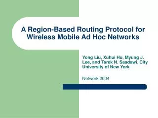
O C T O P U S Scalable Routing Protocol For Wireless Ad Hoc Networks. - Lily Itkin - Evgeny Gurevich - Inna Vaisband -. Lab Chief Engineer: Dr. Ilana David Instructor: Roie Melamed. Location Based Routing Protocols. Proactive protocols

E N D
O C T O P U SScalable Routing Protocol For Wireless Ad Hoc Networks - Lily Itkin - Evgeny Gurevich - Inna Vaisband - Lab Chief Engineer: Dr. Ilana David Instructor: Roie Melamed
Location Based Routing Protocols • Proactive protocols • continuously updates the “reachability” information at all the network nodes • when a route is requested, it is immediately available • Problem:waste wireless resources for handling frequent updates, especially for large, highly mobile networks • Reactive protocols • discover routes only upon demand • involve some sort of “global search” which can causes a significant delay • Problem:very slow, high overhead for each request • Octopus - Hybrid protocol - combines the advantages of both approaches • Cheap maintenance of the proactive part (Core module) • Low-overhead location time - reactive part (FL module) • Simple protocol
100 200 300 400 500 600 100 200 300 400 Octopus’ Grid • The space is divided to horizontal and vertical stripsThe division is related to a (0,0) point and not affected by the nodes’ locations • Each node knows its vertical and horizontal strips a b c d e j f g h i
100 200 300 400 500 600 100 200 300 400 Core Module: The Neighbor List(proactive part) • Every timeout, each node broadcasts its ID and location. • Each node in a range of 250m receives this message and updates its one-hop neighbor list accordingly. updates the list updates the list updates the list a b c d e j f g h i updatesthe list updates the list
j,e,d,c,b j,e,d,c j,e,d j,e,d,c,b,a 100 200 300 400 500 600 100 200 300 400 Core Module: The Strips DB(proactive part) • End Node j initiates the update of its strip. • At the end, the east table of node a is {b, c, d, e, j}. a b c d e j f g h i
h? 100 200 300 400 500 600 100 200 start communicating h! 300 400 FL Module: Locating the Target(reactive part) • Example: Node b wants to transmit data to node h, whose location node b doesn’t know source h? a b c d e j h! f g h access target
Project Workflow • Analyzing results • building relevant tables/graphs • extracting bottle-neck parameters • Finding Solution • functionality updates/additions • design optimizations • system/algorithm parameters • Simulations • writing scripts • executing scripts Start Point Implementation of the basic algorithm (Project I) • Code Updates • design • implementation • testing
Functionality Updates/Additions Motivation Functionality Updates/Additions Motivation • Low success rates (on large grids): • entries found by Find Location module (found ~ 85%) • reply queries returned to the source node (replied ~ 80%) • targets reached from source (received ~ 65%) • Low success rates (on large grids): • entries found by Find Location module (found ~ 85%) • reply queries returned to the source node (replied ~ 80%) • targets reached from source (received ~ 65%)
Functionality Updates/Additions - contd • Sending directions • [1 direction] x [4 sendings] (default) Four directions (North, South, West, East) are being scanned one after another - one direction at a time • [2 directions] x [2 sendings] (optimization)Four directions are being scanned in pairs (North + South, West + East) • [4 directions] x [1 sending] (optimization) Four directions (North, South, West, East) are being scanned simultaneously • [2 directions] x [4 sendings] (optimization) Eight directions are being scanned in pairs (North + South, North-East + South-West, West + East, South-East + North-West) • [4 directions] x [2 sendings] (optimization) Eight directions are being scanned by quartets (North + South + West + East, North-East + South-West + South-East + North-West)
Functionality Updates/Additions - contd • Considerations • Scanning less directions each time (e.g. 1 x 4, 1 x 8) • increases the average search time • decreases the found success rate, because of the chance that the searched mobile node will move to the area that is not in the currently searched direction • Scanning more directories each time (e.g. 4 x 1, 8 x 1) • overhead in resources • high success rates • Conclusion • The total number of sending directions and number of directions sent simultaneously should be determined according to user’s request and resources
Functionality Updates/Additions - contd • Reply routing modes As soon as the searched node is located, the source should be informed. This can be done in 2 ways: • by GF algorithm (default) • by FL_REPLY algorithm (optimization) • Considerations • Default: the natural way to implement the reply to source is via Geographic Forwarding, because the location of the source is known in the moment of the reply • Problem: the accessibility of the access node from the source via FL ensures the accessibility of the source from the access node via FL (in static mode), but does not necessary means the source will be reached from the access node using GF • Conclusions • The empiric results determined that there is no significant difference between the methods, which means that the problem appears only in very specific configurations
100 200 300 400 500 600 100 GF 200 FL 300 FL FL 400 Functionality Updates/Additions - contd • Example: • Node a (source) wants to send data to node e (target) • Node e (target) located by node d (access) via FL • The reply from node d (access) to node a (source) via GF fails target f e access d source a c b
100 100 200 200 300 300 400 400 100 100 200 200 300 300 Functionality Updates/Additions - contd • source – access – source – target (with reply) the access node replies to the source node, which initiates communication with the target source • Establishing connections modes initiates communicating a target g h access • source – access – target(without reply)request is sent directly from the access node to the target node, which initiates communication with the source source a initiates communicating target g h access
Functionality Updates/Additions - contd • Conclusion • The empiric results determined that the rate of the received packets without reply is significantly higher than the rate of the received packets with reply
Functionality Updates/Additions - contd • Absolute/Estimated LocationThere are several options of treating the location to which data should be sent, considering the mobility of the system nodes: • The specified location is the most reliable, although was supplied some time ago. Data is sent to the specified location (default) • The specified location is not reliable enough. An estimated location is calculated based on specified location, target’s velocity (a vector) and time since the location was supplied. Data is sent to the estimated location (optimization) • Basic assumptions: • The velocity of each node is constant during all time of the simulation. • A node changes direction only when it reaches the randomly predefined destination. • The grid is large enough, so nodes rarely change direction. • Estimation: • The location can estimated once – at the moment the sending is originated • The location can be re-estimated after each hop on the route from sender to the target.
Functionality Updates/Additions - contd • Conclusions • The empiric results determined that sending data to the estimated location gives higher success rates than sending to the original location
Functionality Updates/Additions - contd • Cache • The nodes that are located during reactive requests are stored in cache of the nodes in the route • During the reactive requests, FL/GF are initiated only if the searched node is not found in cache • When cache is activated, the timeout parameter defines when the data stored in cache is valid and when it is not • Conclusions • Naturally the found success rates are higher and the received success rates decrease when cache option is activated • Yet, the economy of the system resources (forwardings per packet) is significant • The final decision is a matter of users’ needs and resources
Functionality Updates/Additions - contd • Core and FL Queues • Each time a node sends a packet it is copied to the relevant queue • When the node makes sure the next hop has received the packet (by “hearing” next hop redirecting the packet), it is deleted from the queue • In case the packet was not deleted from the queue during timeout interval, it is being rescheduled • Motivation • The optimization prevents discontinuances in packet transmission
100 100 200 200 300 300 400 400 100 100 200 200 300 300 Functionality Updates/Additions - contd • Example: disconnection of transmission • the expected receiver gets out of the transmission range => the packet is lost • there are no nodes in the transmission range of the receiver=> the packet is lost sender sender packet lost packet lost h a g a g g receiver receiver receiver
Functionality Updates/Additions - contd • Conclusions • The empiric results determined that all success rates were improved • No resource overhead
100 200 300 400 500 600 100 200 300 FL FL BP BP 400 Functionality Updates/Additions - contd • Bypass – Core and FL • The optimization is used when there are no available nodes (receivers) in the sending direction • When the mode is activated, the sender chooses an alternative route that exceeds the strip limit and bypasses the dead area • The route returns to the original strip as soon as possible a e b d c
Functionality Updates/Additions - contd • Conclusions • The empiric results determined that using bypass optimization improves the success rates. The improvement is most significant in the medium grid spaces
Functionality Updates/Additions - contd • Validate DBThe entry is defined as not a valid neighbor and being deleted from the node’s DB lists (one-hop neighbors and strips) • by Location • When estimated location exceeds the limits of the neighbors lists • Estimated location is being calculated based on the DB current and previous locations • by Time • Timeout after the last update • Conclusions • The empiric results determined that the reliability of the DB is higher when the neighbors lists are validated by Location and by Time
Functionality Updates/Additions - contd • Two-hop neighbor tableAn extra table managed by Core module. • decreases the overhead of the reactive FL module • increases the overhead of the proactive Core module • Results • Slightly higher success rates • Significantly larger data-bases to maintain • Significantly higher overhead per packet • Conclusions • The disadvantages supersede the advantages
Functionality Updates/Additions - contd • Unstable Nodes • the basic assumption that all nodes are available at all times is not accurate • in fact, nodes may turn on and off from time to time due to numerous reasons (low battery, no reception etc) • to analyze real-life connectivity, portions of nodes were defined as not reachable in random intervals of time • Results • as it was expected the success rates are inversely proportional to the number of the non-stable nodes.
Porting to Linux • Motivation: • Failure to run simulations on large grid-spaces • Enabling simulation control from remote location • Testing the results in different environments • Overhead: • Reinstallation of NS2 under Linux environment • Porting of Octopus modules into NS2 under Linux environment • Adjustment of simulations’ scripts to Linux environment • Conclusions • The problem of simulations on large grid-spaces was solved • Simulation results found to be similar in both environments
Development Environment • Platform • The protocol is implemented in NS2, discrete event simulator targeted at networking research • The protocol is written in C++ and OTcl • The test environment written in CShell and Tcl • The protocol and tests are supported in Cygwin and Linux environments • System Parameters • Numerous system parameters were expected to impact simulation results and needed fine-tuning based on empirical experiments • These parameters were defined so that they can be easily changed • Among others, these parameters include Strip Resolution, Queues’ Timeouts, Number of Retransmissions, Proactive Updates Intervals etc.
System Parameters As an example, the Strip Resolution was found to be one of the most important parameters to influence on success rates
Simulations • The following scripts were written in order to automate the process of running experiments • single_test.csh <parameter lists> - responsible for setting the desired configuration, running the experiment several times (for better accuracy), collecting and processing the relevant statistical data • test_all.csh <output file> - contains a list of single_test executions with different parameters • file.tcl • the actual input parameter to the NS2 application • responsible for randomly defining each node’s route on the grid during simulation • dynamically updated by single_test on each execution