Download
1 / 70
730 likes | 998 Views
Action Research Measurement Scales and Descriptive Statistics. INFO 515 Glenn Booker. Measurement Needs. Need a long set of measurements for one project, and/or many projects to examine statistical trends Could use measurements to test specific hypotheses

E N D
Action ResearchMeasurement Scales andDescriptive Statistics INFO 515 Glenn Booker Lecture #2
Measurement Needs • Need a long set of measurements for one project, and/or many projects to examine statistical trends • Could use measurements to test specific hypotheses • Other realistic uses of measurement are to help make decisions and track progress • Need scales to make measurements! Lecture #2
Measurement Scales • There are four types of measurement scales • Nominal • Ordinal • Interval • Ratio • Completely optional mnemonic: to remember the sequence, I think of ‘NOIR’ like in the expression ‘film noir’ (‘noir’ is French for ‘black’) Lecture #2
Nominal Scale • A nominal (“name”) scale groups or classifies things into categories, which: • Must be jointly exhaustive (cover everything) • Must be mutually exclusive (one thing can’t be in two categories at once) • Are in any sequence (none better or worse) • So a nominal variable is putting things into buckets which have no inherant order to them Lecture #2
Nominal Scale • Examples include • Gender (though some would dispute limitations of only male/female categories) • Dewey decimal system • The Library of Congress system • Academic majors • Makes of stuff (cars, computers, etc.) • Parts of a system Lecture #2
Ordinal Scale • This measurement ranks things in order • Sequence is important, but the intervals between ranks is not defined numerically • Rank is relative, such as “greater than” or “less than” • E.g. letter grades, urgency of problems, class rank, inspection ratings • So now the buckets we’re using have some sense or order or direction Lecture #2
Interval Scale • An interval scale measures quantitative differences, not just relative • Addition and subtraction are allowed • E.g. common temperature scales (°F or C), a single date (Feb 15, 1999), maybe IQ scores • Let me know if you find any more examples • A zero point, if any, is arbitrary (90 °F is *not* six times hotter than 15 °F!) Lecture #2
Ratio Scale • A ratio scale is an interval scale with a non-arbitrary zero point • Allows division and multiplication • The “best” type of scale to use, if possible • E.g. defect rates for software, test scores, absolute temperature (Kelvin or Rankine), the number or count of almost anything, size, speed, length, … Lecture #2
Summary of Scales • Nominal • names different categories, not ordered, not ranked: Male, Female, Republican, Catholic.. • Ordinal • Categories are ordered: Low, High, Sometimes, Never, • Interval • Fixed intervals, no absolute zero: IQ, Temperature • Ratio • Fixed intervals with an absolute zero point: Age, Income, Years of Schooling, Hours/Week, Weight • Age could be measured as ratio (years), ordinal (young, middle, old), or nominal (baby boomer, gen X) • Scale of measurement affects (may determine) type of statistics that you can use to analyze the data Lecture #2
Scale Hierarchy • Measurement scales are hierarchical:ratio (best) / interval / ordinal / nominal • Lower level scales can always be derived from data which uses a higher scale • E.g. defect rates (a ratio scale) could be converted to {High, Medium, Low} or {Acceptable, Not Acceptable} (ordinal scales) Lecture #2
Reexamine Central Tendencies • If data are nominal, only the mode is meaningful • If data are ordinal, both median and mode may be used • If data are ratio or interval (called “scale” in SPSS), you may use mean, median, and mode Lecture #2
Reexamine Variables • Discrete variables use counting units or specific categories • Example: makes of cars, grades, … • Use Nominal or Ordinal scales • Continuous = Integer or Real Measurements • Example: IQ Test scores, length of a table, your weight, etc. • Use Ratio or Interval scales Lecture #2
Refine Research Types • Qualitative Research tends to use Nominal and/or Ordinal scale variables • Quantitative Research tends to use Interval and/or Ratio scale variables Lecture #2
Frequency Distributions • Frequency distributions describe how many times each value occurs in a data set • They are useful for understanding the characteristics of a data set • Frequencies are the count of how many times each possible value appears for a variable (gender = male, or operating system = Windows 2000) Lecture #2
Frequency Distributions • They are most useful when there is a fixed and relatively small number of options for that variable • They’re harder to use for variables which are numbers (either real or integer) unless there are only a few specific options allowed (e.g. test responses 1 to 5 for a multiple choice question) Lecture #2
Generating Frequency Distributions • Select the command Analyze / Descriptive Statistics / Frequencies… • Select one or more “Variable(s):” • Note that the Frequency (count) and percent are included by default; other outputs may be selected under the “Statistics...” button • A bar chart can be generated as well using the “Charts…” button; see another way later Lecture #2
Sample Frequency Output Lecture #2
Analysis of Frequency Output • The first, unlabeled column has the values of data – here, it first lists all Valid values (there are no Invalid ones, or it would show those too) • The Frequency column is how many times that value appears in the data set • The Percent column is the percent of cases with that value; in the fourth row, the value 15 appears 116 times, which is 24.5% of the 474 total cases (116/474*100 = 24.5%) Lecture #2
Round-off error Analysis of Frequency Output • The Valid Percent column divides each Frequency by the total number of Valid cases (= Percent column if all cases valid) • The Cumulative Percent adds up the Valid Percent values going down the rows; so the first entry is the Valid Percent for first row, the second entry is from 11.2 + 40.1 = 51.3%, next is 51.3 + 1.3 = 52.5% and so on Lecture #2
Generating Frequency Graphs • Frequency is often shown using a bar graph • Bar graphs help make small amounts of data more visible • To generate a frequency graph alone • Click on the Charts menu and select “Bar…” • Leave the “Simple” graph selected, and leave “Summaries are for groups of cases” selected; click the “Define” button Lecture #2
Generating Frequency Graphs • Let the Bars Represent remain “N of cases” • Click on variable “Educational Level (years)” and move it into the Category Axis field • Click “OK” • You should get the graph on the next slide.Notice that the text below the X axis is the Label for the Category Axis. Lecture #2
Sample Frequency Output Notice that the exact same graph can be generated from Frequencies, or just as a bar graph Lecture #2
Frequency Distributions • A frequency distribution is a tabulation that indicates the number of times a score or group of scores occurs • Bar charts best used to graph frequency of nominal & ordinal data • Histograms best used to display shape of interval & ratio data Lecture #2
Frequency Distribution Example SPSS for Windows, Student Version Lecture #2
Basic Measures - Ratio • Used for two exclusive populations (every case fits into one OR the other) • Ratio = (# of testers) / (# of developers) • E.g. tester to developer ratio is 1:4 Lecture #2
Proportions and Fractions • Used for multiple (> 2) populations • Proportion = (Number of this population) / (Total number of all populations) • Sum of all proportions equals unity (one) • E.g. survey results • Proportions are based on integer units • Fractions are based on real numbered units Lecture #2
Percentage • A proportion or fraction multiplied by 100 becomes a percentage • Only report percentages when N (total population measured) is above ~30 to 50; and always provide N for completeness • Why? Otherwise a percentage will imply more accuracy than the data supports • If 2 out of 3 people like something, it’s misleading to report that 66.667% favor it Lecture #2
Percents • Percent = the percentage of cases having a particular value. • Raw percent = divide the frequency of the value by the total number of cases (including missing values) • Valid percent = calculated as above but excluding missing values Lecture #2
Percent Change • The percent increase in a measurement is the new value, minus the old one, divided by the old value; negative means decrease:% increase = (new - old) / old • The percent change is the absolute value of the percent increase or decrease:% change = | % increase | Lecture #2
Percent Increase • Later Value – Earlier Value Earlier Value • So if a collection goes from 50,000 volumes in 1965 to 150,000 in 1975, the percent increase is: • 150,000-50,000 = 2 = 200% 50,000 • Always divide by where you started Carpenter and Vasu, (1978) Lecture #2
Percentiles • A percentile is the point in a distribution at or below a given percentage of scores. • The median is the 50% percentile • Think of the SAT scores - what percentile were you for verbal, math, etc. - means what percent of people did worse than you Lecture #2
Rate • Rate conveys the change in a measurement, such as over time, dx/dt. Rate = (# observed events) / (# of opportunities)*constant • Rate requires exposure to the risk being measured • E.g. defects per KSLOC (1000 lines of code) = (# defects)/(# of KSLOC)*1000 Lecture #2
Exponential Notation • You might see output of the form +2.78E-12 • The ‘E’ means ‘times ten to the power of’ • This is +2.78 * 10-12 (+2.78*10**-12) • A negative exponent, e.g. –12, makes it a very small number • 10-12 = 0.000000000001 • 10+12 = 1,000,000,000,000 • The leading number, here +2.78, controls whether it is a positive or negative number Lecture #2
Exponential Notation +5*10**+12 (a positive number >>1) Pos. +5*10**-12 (a positive number <<1) 0 -5*10**-12 (a negative number <<1) Neg. -5*10**+12 (a negative number >>1) Lecture #2
Precision • Keep your final output to a consistent level of precision (significant digits) • Don’t report one value as “12” and another as “11.86257523454574123” • Pick a level of precision to match the accuracy of your inputs (or one digit more), and make sure everything is reported that way consistently (e.g. 12.0 and 11.9) Lecture #2
Data Analysis • Raw data is collected, such as the dates a particular problem was reported and closed • Refined data is extracted from raw data, e.g. the time it took a problem to be resolved • Derived data is produced by analyzing refined data, such as the average time to resolve problems Lecture #2
Descriptive Statistics • Descriptive statistics describes the key characteristics of one set of data (univariate) • Mean, median, mode, range (see also last week) • Standard deviation, variance • Skewness • Kurtosis • Coefficient of variation Lecture #2
Mean • A.k.a.: Average Score • The mean is the arithmetic average of the scores in a distribution • Add all of the scores • Divide by the total number of scores • The mean is greatly influenced by extreme scores; they pull it off center Lecture #2
Mean Calculation HOLDINGS IN 7 DIFFERENT LIBRARIES X Mean = X N 7400 6500 39200 = 5600 6200 7 5900 5100 4300 Here, sum every data value 3800 X= 39200 Lecture #2
Mean with a Frequency Distribution X (IQ)F=FreqFX = F*X 140 2 280 135 1 135 132 2 264 130 1 130 128 1 128 126 1 126 125 4 500 123 1 123 120 4 480 110 3 330 101 1101 21 2597 Mean =∑FX = 2597 = 123.67 = 124 (round off) N 21 N = SF Lecture #2
Central Tendency Example Staff Salaries $4100 6000 6000 Mode = $6000 6000 8000 Median = 9 + 1 = 5th value = $8000 9000 2 10000 11000 Mean = ∑X = 80100 = $8900 20000 N 9 Carpenter and Vasu, (1978) Lecture #2
Handling Extreme Values • In cases where you have an extreme value (high or low) in a distribution, it is helpful to report both the median and the mean • Reporting both values gives some indication (through comparison) of a skewed distribution Lecture #2
Measures of Variation • Measures which indicate the variation, or spread of scores in a distribution • Range (see last week) • Variance • Standard Deviation Lecture #2
Standard Deviation, Variance • Standard deviation is the average amount the data differs from the mean (average)SD = ( S (Xi-X)**2 / (N-1) )SD = ( Variance ) • Variance is the standard deviation squaredVariance = S (Xi-X)**2 / (N-1) [per ISO 3534-1, para 2.33 and 2.34] Lecture #2
Standard Deviation • The standard deviation is the square root of the variance. It is expressed in the same units as the original data. • Since the variance was expressed “squared units” it doesn’t make much practical sense. For example, what are “squared books” or “squared man-hours?” Lecture #2
Computing the VarianceS2 = ∑(X – Mean)2 N • 1. Subtract the mean from each score • 2. Square the result • 3. Sum the squares for all data points • 4. Divide by the N of cases Lecture #2
Divide by N or N-1??? • You’ll see different formulas for variance and standard deviation – some divide by N, some by N-1 (e.g. slides 43 and 45); why? • If your data covers the entire population (you have all of the possible data to analyze), then divide by N • If your data covers a sample from the population, divide by N-1 Lecture #2
Standard Deviation for Freq Dist. XFFXX2FX2 17 2 34 289 578 16 4 64 256 1024 14 5 70 196 980 10 2 20 100 200 9 3 27 81 243 6 1 6 36 36 221 3061 σ = √ (∑FX2 – (∑FX)2/N) = √ (3061- (221)2/17) N 17 = √ ((3061- 2873)/17) = 3.3 Notice that FX2is F*(X2), not (F*X)2 Standard Deviation of Bookmobile Distribution Lecture #2
Std Dev Reflects Consistency Distance from Target Frequency In MetersBattery ABattery B 200 2 0 150 4 1 100 5 5 50 7 10 0 9 13 -50 7 10 -100 5 5 -150 4 1 -200 2 0 Mean =0 Mean =0 Standard D. = Standard D. = 102.74 65.83 Runyon and Haber (1984) Lecture #2
Standard Deviation vs. Std. Error • To be precise, the standard error is the standard deviation of a statistic used to estimate a population parameter [per ISO 3534-1, para 2.56 and 2.50] • So standard error pertains to sample data, while standard deviation should describe the entire population • We often use them interchangeably Lecture #2