Download
1 / 19
190 likes | 270 Views
Automated indicator of local variation in vegetal cover Estevan Barbará Teixeira José Augusto Sapienza Ramos Laboratório de Geotecnologias 2011, August 19 th. Objectives. To study a method of statistical analysis of vegetation cover variation through time.

E N D
Automated indicator of local variation in vegetal cover Estevan Barbará Teixeira José Augusto Sapienza Ramos Laboratório de Geotecnologias 2011, August 19th
Objectives • To study a method of statistical analysis of vegetation cover variation through time. • To implement the method using a user-friendly free software
Motivation • More people have access to remote sensing imagery. • Some of these people make decisions based on the data. • The data by itself frequently isn’t enough, demanding analysis. • The methods of evaluation require technical knowledge. • This work proposes an automated analysis of the vegetation index variation to monitor vegetal cover and other changings.
Concepts • Vegetation Index • A calculation of the vegetation rate in a sample of eletromagnetical radiation, such as a raster image generated by a sensor. • Many vegetation indices uses the radiation of the red and near-infrared bands of eletromagnetical spectre. • The red radiation reflects poorly on the clorophyll of green leaves, and the nirradiation is highly reflected by the leaf cell’s shapes.
NDVI • Index choosed to our work; • Acronym of Normalized Differences Vegetation Index; • One of the most used vegetation indices; • Its calculation is based on the formula: • The results varies between -1 and 1.
NDVI • The low results indicates lack of clorophyll and aditionally, likely presence of exposed soil, or water bodies. • The high results indicates high population of features rich in clorophyll, such as green leaves.
Image preparations • The remote sensor’s images are not immediatelly suitable to the NDVI calculation, because of the following factors: • There is some distortion between the eletromagnetic radiation rate that hits the ground and the rate caught by the sensor. • The sensor converts the levels of radiation measured into a digital number, with a particular formula for each sensor calibration.
Imagepreparations – Step1 (SpectralRadiance) • Firstly, the digital number of the pixel (an integer number, for instance, between 0 and 255 in the TM/Landsat sensors.) must be converted on the actual radiance value.
Image preparations – Step 2 (TOA Reflectance) • After, from the radiance reflected at the surface must be calculated the radiance reflected at the top of atmosphere. • The formula uses as variables • the spectral radiance (Ll), • the distance between the Earth and Sun (d), • the mean solar irradiance of the sensor band (ESUNl), • and the solar zenithal angle (qs)
Indicator of NDVI changes • The NDVI variation between different dates can be used to asess the gain or loss of vegetation. • This variation may be caused by fires or deforestation, but also by season changes, plantings and harvests, or atmospherical conditions.
Indicator of NDVI changes • So, this indicator purposes the use of statistical analysis to evaluate the index variation. • The variation is analyzed using its standard deviation.
The software • The algorithm was modelled in a software, which only demands: • The satellite images (specifically, the red and nir bands). • The date of the images. • The solar zenith angle. • A b parameter to adjust the number of standard deviations of the statistic calculation.
Example: Legal Amazon limits and neighborhood, Tocantins state (b = 1.5) 2009, June 14th 2010, June 17th Image result of the method
Example: Neighborhood of Uberaba, Minas Gerais state (b = 0.5) 2010, June 27th 2010, September 7th Image result of the method
Example: Flooding area of Salto Caxias hydroeletric plant, Paraná state (b = 2) 1996, June 10th 1999, May 2nd Image result of the method
Example: Neighborhood of Floresta, Pernambuco state (b = 1) 1994, May 19th 2001, May 6th Image result of the method
Conclusions • From 10 cases tested, we found that: • More tests are clearly needed to the method evaluation. • The method responds well to agriculture and fires. • In some cases, however, the method doesn’t show good results with rivers and/or clouds. • The automated method shows to be suitable to a quick evaluation of some factors. • For more detailed analysis are needed other methods.
Next works • Research ways to solve problems arised from many sources, specially image overlap and georeferencing. • Studies of the application of image filters are under way. • The software is being adapted to plugin for QuantumGIS and ArcGIS.
Thank You Estevan Barbará Teixeira - ebarbara@labgis.uerj.br José Augusto Sapienza Ramos - sapienza@labgis.uerj.br