Relational Database Design

1. Relational Database Design

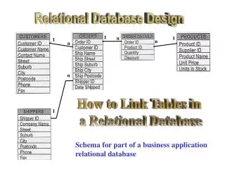
2. Relational Database Design • Features of Good Relational Design • Atomic Domains and First Normal Form • Decomposition Using Functional Dependencies • Functional Dependency Theory • Algorithms for Functional Dependencies • Normal Form • Database-Design Process • Modeling Temporal Data

3. The Banking Schema • branch = (branch_name, branch_city, assets) • customer = (customer_id, customer_name, customer_street, customer_city) • loan = (loan_number, amount) • account = (account_number, balance) • employee = (employee_id. employee_name, telephone_number, start_date) • dependent_name = (employee_id, dname) • account_branch = (account_number, branch_name) • loan_branch = (loan_number, branch_name) • borrower = (customer_id, loan_number) • depositor = (customer_id, account_number) • cust_banker = (customer_id, employee_id, type) • works_for = (worker_employee_id, manager_employee_id) • payment = (loan_number, payment_number, payment_date, payment_amount) • savings_account = (account_number, interest_rate) • checking_account = (account_number, overdraft_amount)

4. Combine Schemas? • Suppose we combine borrower and loan to get bor_loan = (customer_id, loan_number, amount ) • Result is possible repetition of information (L-100 in example below)

5. A Combined Schema Without Repetition • Consider combining loan_branch and loan loan_amt_br = (loan_number, amount, branch_name) • No repetition (as suggested by example below)

6. What About Smaller Schemas? • Suppose we had started with bor_loan. How would we know to split up (decompose) it into borrower and loan? • Write a rule “if there were a schema (loan_number, amount), then loan_number would be a candidate key” • Denote as a functional dependency: loan_numberamount • In bor_loan, because loan_number is not a candidate key, the amount of a loan may have to be repeated. This indicates the need to decompose bor_loan. • Not all decompositions are good. Suppose we decompose employee into employee1 = (employee_id, employee_name) employee2 = (employee_name, telephone_number, start_date) • The next slide shows how we lose information -- we cannot reconstruct the original employee relation -- and so, this is a lossy decomposition.

7. A Lossy Decomposition

8. First Normal Form • Domain is atomic if its elements are considered to be indivisible units • Examples of non-atomic domains: • Set of names, composite attributes • Identification numbers like CS101 that can be broken up into parts • A relational schema R is in first normal form if the domains of all attributes of R are atomic • Non-atomic values complicate storage and encourage redundant (repeated) storage of data • Example: Set of accounts stored with each customer, and set of owners stored with each account

9. First Normal Form (Cont’d) • Atomicity is actually a property of how the elements of the domain are used. • Example: Strings would normally be considered indivisible • Suppose that students are given roll numbers which are strings of the form CS0012 or EE1127 • If the first two characters are extracted to find the department, the domain of roll numbers is not atomic. • Doing so is a bad idea: leads to encoding of information in application program rather than in the database.

10. Goal — Devise a Theory for the Following • Decide whether a particular relation R is in “good” form. • In the case that a relation R is not in “good” form, decompose it into a set of relations {R1, R2, ..., Rn} such that • each relation is in good form • the decomposition is a lossless-join decomposition • Our theory is based on: • functional dependencies • multivalued dependencies

11. Functional Dependencies • Constraints on the set of legal relations. • Require that the value for a certain set of attributes determines uniquely the value for another set of attributes. • A functional dependency is a generalization of the notion of a key.

12. Functional Dependencies (Cont.) • Let R be a relation schema   R and   R • The functional dependency  holds onR if and only if for any legal relations r(R), whenever any two tuples t1and t2 of r agree on the attributes , they also agree on the attributes . That is, t1[] = t2 []  t1[ ] = t2 [ ] • Example: Consider r(A,B ) with the following instance of r. • On this instance, AB does NOT hold, but BA does hold. • 4 • 1 5 • 3 7

13. Functional Dependencies (Cont.) • K is a superkey for relation schema R if and only if K R • K is a candidate key for R if and only if • K R, and • for no   K,  R • Functional dependencies allow us to express constraints that cannot be expressed using superkeys. Consider the schema: bor_loan = (customer_id, loan_number, amount ). We expect this functional dependency to hold: loan_numberamount but would not expect the following to hold: amount customer_name

14. Use of Functional Dependencies • We use functional dependencies to: • test relations to see if they are legal under a given set of functional dependencies. • If a relation r is legal under a set F of functional dependencies, we say that rsatisfies F. • specify constraints on the set of legal relations • We say that Fholds onR if all legal relations on R satisfy the set of functional dependencies F. • Note: A specific instance of a relation schema may satisfy a functional dependency even if the functional dependency does not hold on all legal instances. • For example, a specific instance of loan may, by chance, satisfy amount customer_name.

15. Functional Dependencies (Cont.) • A functional dependency is trivial if it is satisfied by all instances of a relation • Example: • customer_name, loan_number customer_name • customer_name customer_name • In general,   is trivial if   

16. Closure of a Set of Functional Dependencies • Given a set F of functional dependencies, there are certain other functional dependencies that are logically implied by F. • For example: If AB and BC, then we can infer that AC • The set of all functional dependencies logically implied by F is the closure of F. • We denote the closure of F by F+. • F+ is a superset of F.

17. Boyce-Codd Normal Form A relation schema R is in BCNF with respect to a set F of functional dependencies if for all functional dependencies in F+ of the form  where  R and  R,at least one of the following holds: •  is trivial (i.e.,  ) •  is a superkey for R Example schema not in BCNF: bor_loan = ( customer_id, loan_number, amount ) because loan_numberamount holds on bor_loan but loan_number is not a superkey

18. Decomposing a Schema into BCNF • Suppose we have a schema R and a non-trivial dependency causes a violation of BCNF. We decompose R into: • (U ) • ( R - (  -  ) ) • In our example, •  = loan_number •  = amount and bor_loan is replaced by • (U ) = ( loan_number, amount ) • ( R - (  -  ) ) = ( customer_id, loan_number )

19. BCNF and Dependency Preservation • Constraints, including functional dependencies, are costly to check in practice unless they pertain to only one relation • If it is sufficient to test only those dependencies on each individual relation of a decomposition in order to ensure that all functional dependencies hold, then that decomposition is dependency preserving. • Because it is not always possible to achieve both BCNF and dependency preservation, we consider a weaker normal form, known as third normal form.

20. Third Normal Form • A relation schema R is in third normal form (3NF) if for all:  in F+at least one of the following holds: • is trivial (i.e.,  ) •  is a superkey for R • Each attribute A in  –  is contained in a candidate key for R. (NOTE: each attribute may be in a different candidate key) • If a relation is in BCNF it is in 3NF (since in BCNF one of the first two conditions above must hold). • Third condition is a minimal relaxation of BCNF to ensure dependency preservation (will see why later).

21. Goals of Normalization • Let R be a relation scheme with a set F of functional dependencies. • Decide whether a relation scheme R is in “good” form. • In the case that a relation scheme R is not in “good” form, decompose it into a set of relation scheme {R1, R2, ..., Rn} such that • each relation scheme is in good form • the decomposition is a lossless-join decomposition • Preferably, the decomposition should be dependency preserving.

22. How good is BCNF? • There are database schemas in BCNF that do not seem to be sufficiently normalized • Consider a database classes (course, teacher, book ) such that (c, t, b)  classes means that t is qualified to teach c, and b is a required textbook for c • The database is supposed to list for each course the set of teachers any one of which can be the course’s instructor, and the set of books, all of which are required for the course (no matter who teaches it).

23. How good is BCNF? (Cont.) course teacher book • There are no non-trivial functional dependencies and therefore the relation is in BCNF • Insertion anomalies – i.e., if Marilyn is a new teacher that can teach database, two tuples need to be inserted (database, Marilyn, DB Concepts) (database, Marilyn, Ullman) database database database database database database operating systems operating systems operating systems operating systems Avi Avi Hank Hank Sudarshan Sudarshan Avi Avi Pete Pete DB Concepts Ullman DB Concepts Ullman DB Concepts Ullman OS Concepts Stallings OS Concepts Stallings classes

24. How good is BCNF? (Cont.) • Therefore, it is better to decompose classes into: course teacher database database database operating systems operating systems Avi Hank Sudarshan Avi Jim teaches course book database database operating systems operating systems DB Concepts Ullman OS Concepts Shaw text This suggests the need for higher normal forms, such as Fourth Normal Form (4NF), which we shall see later.

25. Functional-Dependency Theory • We now consider the formal theory that tells us which functional dependencies are implied logically by a given set of functional dependencies. • We then develop algorithms to generate lossless decompositions into BCNF and 3NF • We then develop algorithms to test if a decomposition is dependency-preserving

26. Closure of a Set of Functional Dependencies • Given a set F set of functional dependencies, there are certain other functional dependencies that are logically implied by F. • For example: If AB and BC, then we can infer that A C • The set of all functional dependencies logically implied by F is the closure of F. • We denote the closure of F by F+. • We can find all ofF+by applying Armstrong’s Axioms: • if   , then   (reflexivity) • if  , then    (augmentation) • if  , and   , then   (transitivity) • These rules are • sound (generate only functional dependencies that actually hold) and • complete (generate all functional dependencies that hold).

27. Example • R = (A, B, C, G, H, I)F = { A BA CCG HCG IB H} • some members of F+ • A H • by transitivity from A B and B H • AG I • by augmenting A C with G, to get AG CG and then transitivity with CG I • CG HI • by augmenting CG I to infer CG  CGI, and augmenting of CG H to inferCGI HI, and then transitivity

28. To compute the closure of a set of functional dependencies F: F + = Frepeatfor each functional dependency f in F+ apply reflexivity and augmentation rules on fadd the resulting functional dependencies to F +for each pair of functional dependencies f1and f2 in F +iff1 and f2 can be combined using transitivitythen add the resulting functional dependency to F +until F + does not change any further NOTE: We shall see an alternative procedure for this task later Procedure for Computing F+

29. Closure of Functional Dependencies (Cont.) • We can further simplify manual computation of F+ by using the following additional rules. • If   holds and  holds, then    holds (union) • If    holds, then   holds and  holds (decomposition) • If   holds and   holds, then   holds (pseudotransitivity) The above rules can be inferred from Armstrong’s axioms.

30. Closure of Attribute Sets • Given a set of attributes a, define the closureof aunderF (denoted by a+) as the set of attributes that are functionally determined by a under F • Algorithm to compute a+, the closure of a under F result := a;while (changes to result) do for each in F do begin if  result then result := result end

31. Example of Attribute Set Closure • R = (A, B, C, G, H, I) • F = {A BA C CG HCG IB H} • (AG)+ 1. result = AG 2. result = ABCG (A C and A  B) 3. result = ABCGH (CG H and CG  AGBC) 4. result = ABCGHI (CG I and CG  AGBCH) • Is AG a candidate key? • Is AG a super key? • Does AG R? == Is (AG)+  R • Is any subset of AG a superkey? • Does AR? == Is (A)+  R • Does GR? == Is (G)+  R

32. There are several uses of the attribute closure algorithm: Testing for superkey: To test if  is a superkey, we compute +, and check if +contains all attributes of R. Testing functional dependencies To check if a functional dependency    holds (or, in other words, is in F+), just check if   +. That is, we compute +by using attribute closure, and then check if it contains . Is a simple and cheap test, and very useful Computing closure of F For each   R, we find the closure +, and for each S  +, we output a functional dependency   S. Uses of Attribute Closure

33. Canonical Cover • Sets of functional dependencies may have redundant dependencies that can be inferred from the others • For example: A  C is redundant in: {AB, BC} • Parts of a functional dependency may be redundant • E.g.: on RHS: {AB, BC, ACD} can be simplified to {A B, BC, AD} • E.g.: on LHS: {A B, BC, ACD} can be simplified to {A B, BC, AD} • Intuitively, a canonical cover of F is a “minimal” set of functional dependencies equivalent to F, having no redundant dependencies or redundant parts of dependencies

34. Extraneous Attributes • Consider a set F of functional dependencies and the functional dependency   in F. • Attribute A is extraneous in  if A   and F logically implies (F – {})  {( – A) }. • Attribute A is extraneous in  if A  and the set of functional dependencies (F – {})  {(– A)} logically implies F. • Note: implication in the opposite direction is trivial in each of the cases above, since a “stronger” functional dependency always implies a weaker one • Example: Given F = {AC, ABC } • B is extraneous in AB C because {AC, AB C} logically implies AC (I.e. the result of dropping B from AB C). • Example: Given F = {AC, ABCD} • C is extraneous in ABCD since AB C can be inferred even after deleting C

35. Testing if an Attribute is Extraneous • Consider a set F of functional dependencies and the functional dependency   in F. • To test if attribute A   is extraneousin • compute ({} – A)+ using the dependencies in F • check that ({} – A)+ contains ; if it does, A is extraneous in • To test if attribute A  is extraneous in  • compute + using only the dependencies in F’ = (F – {})  {(– A)}, • check that + contains A; if it does, A is extraneous in 

36. Canonical Cover • A canonical coverfor F is a set of dependencies Fc such that • F logically implies all dependencies in Fc, and • Fclogically implies all dependencies in F, and • No functional dependency in Fccontains an extraneous attribute, and • Each left side of functional dependency in Fcis unique. • To compute a canonical cover for F:repeatUse the union rule to replace any dependencies in F11 and 12 with 112 Find a functional dependency  with an extraneous attribute either in  or in  If an extraneous attribute is found, delete it from until F does not change • Note: Union rule may become applicable after some extraneous attributes have been deleted, so it has to be re-applied

37. Computing a Canonical Cover • R = (A, B, C)F = {A BC B C A BABC} • Combine A BC and A B into A BC • Set is now {A BC, B C, ABC} • A is extraneous in ABC • Check if the result of deleting A from ABC is implied by the other dependencies • Yes: in fact, BC is already present! • Set is now {A BC, B C} • C is extraneous in ABC • Check if A C is logically implied by A B and the other dependencies • Yes: using transitivity on A B and B  C. • Can use attribute closure of A in more complex cases • The canonical cover is: A B B C

38. Lossless-join Decomposition • For the case of R = (R1, R2), we require that for all possible relations r on schema R r = R1(r ) R2(r ) • A decomposition of R into R1 and R2 is lossless join if and only if at least one of the following dependencies is in F+: • R1 R2R1 • R1 R2R2

39. Example • R = (A, B, C)F = {A B, B C) • Can be decomposed in two different ways • R1 = (A, B), R2 = (B, C) • Lossless-join decomposition: R1  R2 = {B}and B BC • Dependency preserving • R1 = (A, B), R2 = (A, C) • Lossless-join decomposition: R1  R2 = {A}and A  AB • Not dependency preserving (cannot check B C without computing R1 R2)

40. Dependency Preservation • Let Fibe the set of dependencies F + that include only attributes in Ri. • A decomposition is dependency preserving, if (F1 F2  …  Fn )+ = F + • If it is not, then checking updates for violation of functional dependencies may require computing joins, which is expensive.

41. To check if a dependency    is preserved in a decomposition of R into R1, R2, …, Rn we apply the following test (with attribute closure done with respect to F) result = while (changes to result) dofor eachRiin the decompositiont = (result  Ri)+  Riresult = result  t If result contains all attributes in , then the functional dependency    is preserved. We apply the test on all dependencies in F to check if a decomposition is dependency preserving This procedure takes polynomial time, instead of the exponential time required to compute F+and(F1 F2  …  Fn)+ Testing for Dependency Preservation

42. Example • R = (A, B, C )F = {AB B  C}Key = {A} • R is not in BCNF • Decomposition R1 = (A, B), R2 = (B, C) • R1and R2 in BCNF • Lossless-join decomposition • Dependency preserving

43. Comparison of BCNF and 3NF • It is always possible to decompose a relation into a set of relations that are in 3NF such that: • the decomposition is lossless • the dependencies are preserved • It is always possible to decompose a relation into a set of relations that are in BCNF such that: • the decomposition is lossless • it may not be possible to preserve dependencies.

44. Design Goals • Goal for a relational database design is: • BCNF. • Lossless join. • Dependency preservation. • If we cannot achieve this, we accept one of • Lack of dependency preservation • Redundancy due to use of 3NF • Interestingly, SQL does not provide a direct way of specifying functional dependencies other than superkeys. Can specify FDs using assertions, but they are expensive to test • Even if we had a dependency preserving decomposition, using SQL we would not be able to efficiently test a functional dependency whose left hand side is not a key.

45. Overall Database Design Process • We have assumed schema R is given • R could have been generated when converting E-R diagram to a set of tables. • R could have been a single relation containing all attributes that are of interest (called universal relation). • Normalization breaks R into smaller relations. • R could have been the result of some ad hoc design of relations, which we then test/convert to normal form.

46. ER Model and Normalization • When an E-R diagram is carefully designed, identifying all entities correctly, the tables generated from the E-R diagram should not need further normalization. • However, in a real (imperfect) design, there can be functional dependencies from non-key attributes of an entity to other attributes of the entity • Example: an employee entity with attributes department_number and department_address, and a functional dependency department_number  department_address • Good design would have made department an entity • Functional dependencies from non-key attributes of a relationship set possible, but rare --- most relationships are binary

47. Denormalization for Performance • May want to use non-normalized schema for performance • For example, displaying customer_name along with account_number and balance requires join of account with depositor • Alternative 1: Use denormalized relation containing attributes of account as well as depositor with all above attributes • faster lookup • extra space and extra execution time for updates • extra coding work for programmer and possibility of error in extra code • Alternative 2: use a materialized view defined as account depositor • Benefits and drawbacks same as above, except no extra coding work for programmer and avoids possible errors

48. Other Design Issues • Some aspects of database design are not caught by normalization • Examples of bad database design, to be avoided: Instead of earnings (company_id, year, amount ), use • earnings_2004, earnings_2005, earnings_2006, etc., all on the schema (company_id, earnings). • Above are in BCNF, but make querying across years difficult and needs new table each year • company_year(company_id, earnings_2004, earnings_2005, earnings_2006) • Also in BCNF, but also makes querying across years difficult and requires new attribute each year. • Is an example of a crosstab, where values for one attribute become column names • Used in spreadsheets, and in data analysis tools

49. Modeling Temporal Data • Temporal data have an association time interval during which the data are valid. • A snapshot is the value of the data at a particular point in time • Several proposals to extend ER model by adding valid time to • attributes, e.g. address of a customer at different points in time • entities, e.g. time duration when an account exists • relationships, e.g. time during which a customer owned an account • But no accepted standard • Adding a temporal component results in functional dependencies like customer_id  customer_street, customer_city not to hold, because the address varies over time • A temporal functional dependency X  Y holds on schema R if the functional dependency X  Y holds on all snapshots for all legal instances r (R ) t

50. Modeling Temporal Data (Cont.) • In practice, database designers may add start and end time attributes to relations • E.g. course(course_id, course_title)  course(course_id, course_title, start, end) • Constraint: no two tuples can have overlapping valid times • Hard to enforce efficiently • Foreign key references may be to current version of data, or to data at a point in time • E.g. student transcript should refer to course information at the time the course was taken