Download
1 / 27
270 likes | 412 Views
Blood Glucose Prediction using Physiological Models and Support Vector Regression. Razvan Bunescu Nigel Struble Cindy Marling. Frank Schwartz Jay Shubrook. Ohio University, Athens, OH. Management of Type I Diabetes. Approximately 20 million people have Type 1 Diabetes:

E N D
Blood Glucose Prediction using Physiological Models and Support Vector Regression Razvan Bunescu Nigel Struble Cindy Marling Frank Schwartz Jay Shubrook Ohio University, Athens, OH
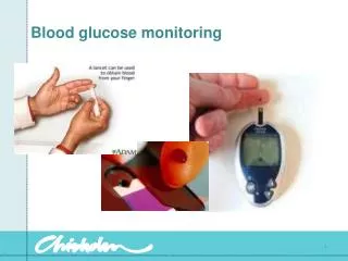
Management of Type I Diabetes • Approximately 20 million people have Type 1 Diabetes: • In type 1 diabetes, the pancreas produces no insulin. • Patients depend upon external supplies of insulin, via injections or insulin pumps. • Diabetes can not be cured, but it can be treated and managed: • To delay or prevent long-term complications, patients try to keep Blood Glucose Levels (BGL) as close to normal as possible. • Patients monitor blood glucose using: • Glucometers (fingerstick measurements). • Continuous Glucose Measurement Systems (CGMS). => loads of data to interpret.
Chronic Complications vs. Blood Glucose Control • Foot Ulcers • Angina • Heart Attack • Coronary Bypass Surgery • Stroke • Kidney Transplant • Dialysis • Blindness • Amputation • Albuminuria • Macular Edema • Proliferative • Retinopathy • Periodontal Disease • Impotence • Gastroparesis • Depression RISK • Microalbuminuria • Mild Retinopathy • Mild Neuropathy CONTROL Good Poor
Continuous Glucose Monitoring (CGM) in Insulin Pump Therapy Systems • CGM Sensor: • interstitial BGL. • every 5 minutes. Insulin Pump delivers insulin through boluses and basal rate:
Achieving Good Blood Glucose Control • Patients must continually monitor their blood glucose levels and adjust insulin doses, striving to keep blood glucose levels as close to normal as possible: • Requires significant effort from patients and doctors. • Try to avoid especially: • Hypoglycemia • Hyperglycemia • Excessive Glycemice Variability forecasting of blood glucose levels detection of glycemic variability
Automatic BGL Prediction • Design a time series forecasting model that predicts BGL 30 or 60 minutes into the future: • Accurate predictions up to 60m in advance would allow plenty of time to take preventive action, to avoid hypo- or hyper-glycemia. • Inputs for the prediction model: • Previous blood glucose measurements taken at 5-minute intervals through a CGM system. • Daily event data: • Insulin dosages, recorded in the CGM device. • Life events, collected through a smartphone interface.
Glucometer Sensor Insulin Bolus Input: Blood Glucose Levels and Insulin Dosages 350 300 250 Glucose (mg/dl) 200 150 100 50 0
Input: Life Events • Developed a smartphone interface to collect relevant life events: • Meals (carb amounts, glycemic index). • Sleep (start, end). • Work (start, end). • Exercise (intensity, start, duration). • Hypoglycemic event. • Health events (stress, depression, ...). • Other events. • Designed to encourage entering events immediately before/after they happen: • to minimize incorrect/incomplete data.
Evaluation Dataset • Total of 1,400 days worth of clinical patient data: • CGMS + insulin + life events. • Human performance on the task of BGL prediction: • Asked 3 diabetes experts to manually label an evaluation dataset with their 30/60 min predictions: • 200 timestamps, coming from 5 patients with T1D. • 40 points per patient. • Manually selected to reflect a diverse set of situations. • Built a GUI to facilitate navigating the data and labeling.
Physician Performance • Compared the 3 physicians against 2 baselines: • t0 predicts that future BGL is the same as current BGL. • AutoRegressive Integrated Moving Averages (ARIMA), trained on past BGL data. • Evaluation measures: • Root Mean Square Error (RMSE). • Total cost of ternary classification: • Future BGL is Same (S), Lower (L), Higher (H) as current BGL. • Same means within 5 (10) mg/dl for 30 (60) min prediction. • cost(L, S) = cost (H, S) = 1; cost(L, H) = 2.
Physician Performance • Physicians, who use daily event data, outperform ARIMA. • Physicians regularly refer to daily events: • Timing of meal events and boluses, carb amouns, bolus types. Use daily events to extract features for automatic BGL prediction.
Physiological Modeling of BG Dynamics • Use equations from literature [6, 7, 8, 9] to model dynamics of variables that are relevant to BG behavior: • Almost identical equations (based on the same data). • Characterize the overall dynamics into 3 compartments: • Meal absorption dynamics. • Insulin dynamics. • Glucose dynamics. • Update some equations and their parameters to better match published data and feedback from our doctors.
A Physiological Model of BG Dynamics • A continuous dynamical model that is described by: • The input variables U. • The state variables X. • The state transition function f that computes the next state given the current state and input i.e. Xt+1 = f(Xt,Ut). • The vector of input variables U contains: • UC(t), the carbohydrate intake measured in grams (g). • UI(t), the amount of insulin measured in insulin units (U): • Computed from bolus events and basal rate data.
A Physiological Model of BG Dynamics • The state variables Xare organized according to the 3 compartments: • Meal Absorption Dynamics: • Cg1(t) = carbohydrate consumption (g). • Cg2(t) = carbohydrate digestion (g). • Insulin Dynamics: • IS(t) = subcutaneous insulin (μU). • Im(t) = insulin mass (μU). • I(t) = level of active plasma insulin (μU/ml). • Glucose Dynamics: • Gm(t) = blood glucose mass (mg). • G(t) = blood glucose concentration (mg).
A Physiological Model of BG Dynamics • The state transition function f captures dependencies among variables in X and U at consecutive time steps:
Glucose Dynamics: Insulin Dependent Utilization Gm(t+1) = Gm(t) − Δdep− Δind − Δclr −Δdep + Δabs + Δegp Δdep = α1 × I(t) × [G(t) + α2]
A Physiological Model of BG Dynamics • The state transition equations were used in an Extended Kalman Filter (EKF) model: • Run a state prediction step every 1 minute. • Run a correction step every 5 minutes. • The EKF model itself can be used to make 30 or 60 minute predictions: • Performance is lower even than the t0 baseline. • Could improve by tunning the α parameters for each patient: • Time consuming, unfeasible due to large number of params. • Difficult to incorporate other types of life events in the model.
A Support Vector Regression (SVR) Model with Physiological Features • The state vector X(t) computed by the physiological model is X(t) = [Cg1(t), Cg2(t), IS(t), Im(t), I(t), Gm(t), G(t)]: • Run the EKF model up to time t0, with a correction step every 5 minutes => X(t0). • Run the EKF model in prediction mode for 60 more minutes => X(t0 + 30) and X(t0 + 60). • Create the following features for the SVR model: • All predicted state variables in X(t0 + 30) andX(t0 + 60). • The difference vectors X(t0) − X(t0 + 30) and X(t0) − X(t0 + 60). • 12 features deltai = BG(t0) − BG(t0 – 5i). • Optionally, train ARIMA on 4 days before t0, and use the 12 predictions in the one hour after t0 as features. 48
SVR Evaluation • Train SVR on the week of data preceding each test point t0: • Use a Gaussian kernel: • Tune parameters γ, ε, and C using grid search on the week preceding the training week. • If not enough tunning examples, use generic parameters tuned on another patient. • Compare the best doctor performance with: • ARIMA and the t0 baselines. • SVR model using physiological features, with (SVRφ+A) and without (SVRφ) ARIMA features. • A previous SVR system (SVRπ+A) that uses CGM data, ARIMA, and an ad-hoc implementation of daily event features.
Experimental Results on BGL Prediction Both SVRφ systems outperform the 3 diabetes experts!
Conclusions and Future Work • Built an adaptive model for BGL prediction that outperforms human experts: • Physiological modeling was essential to good performance. • In future work, extend to use richer set of daily events, such as exercise and stress: • Investigate unobtrusive sensing devices in order to reduce the amount of input required from the patient. • Time of day is also important: • Dawn Phenomenon, i.e. early morning increase in BGL.
Acknowledgments • Our dedicated Research Nurses. • Our current and former Graduate Students: • Nattada Nimsuwan (OU), Melih Altun (OU), and Matthew Wiley (UC-Riverside). • Over 50 Anonymous Patients with Type 1 Diabetes on insulin pump therapy. • Our generous sponsors: