Download
1 / 15
160 likes | 347 Views
If your several predictors are categorical , MRA is identical to ANOVA. If your sole predictor is continuous , MRA is identical to correlational analysis. If your sole predictor is dichotomous , MRA is identical to a t-test. Do your residuals meet the required assumptions ?.

E N D
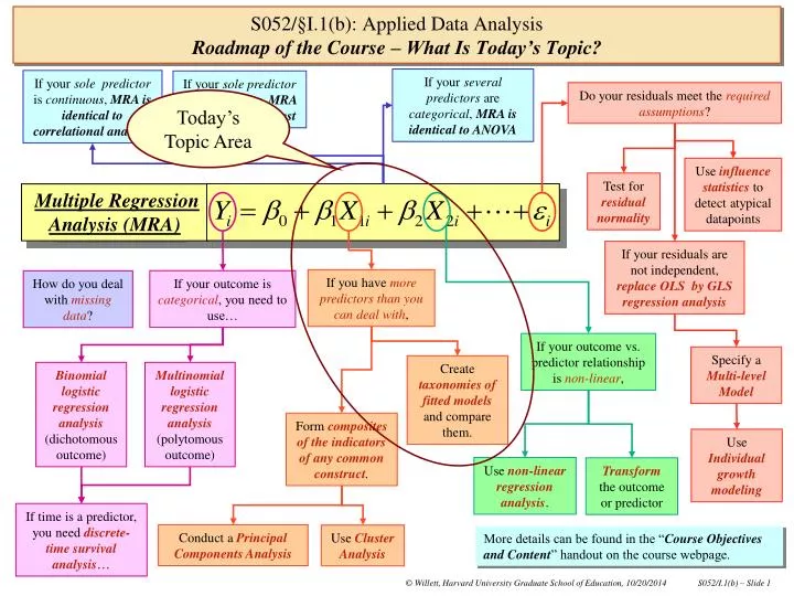
If your several predictors are categorical, MRA is identical to ANOVA If your sole predictor is continuous, MRA is identical to correlational analysis If your solepredictor is dichotomous, MRA is identical to a t-test Do your residuals meet the required assumptions? Today’s Topic Area Use influence statistics to detect atypical datapoints Test for residual normality Multiple Regression Analysis (MRA) If your residuals are not independent, replace OLS byGLS regression analysis If you have more predictors than you can deal with, If your outcome is categorical, you need to use… How do you deal with missing data? If your outcome vs. predictor relationship isnon-linear, Specify a Multi-level Model Create taxonomies of fitted models and compare them. Binomiallogistic regression analysis (dichotomous outcome) Multinomial logistic regression analysis (polytomous outcome) Form composites of the indicators of any common construct. Use Individual growth modeling Use non-linear regression analysis. Transform the outcome or predictor If time is a predictor, you need discrete-time survival analysis… Conduct a Principal Components Analysis Use Cluster Analysis More details can be found in the “Course Objectives and Content” handout on the course webpage. S052/§I.1(b): Applied Data AnalysisRoadmap of the Course – What Is Today’s Topic?
Syllabus Section I.1(b), on Testing Complex Hypotheses About Regression Parameters, includes: • Sometimes you may need to test more complex hypotheses (Slide 3). • Framing a joint hypothesis on several regression parameters simultaneously (Slide 4). • Using the GLH strategy to test a joint hypothesis (Slides 5-7). • Using the GLH test at critical decision points in taxonomy-building (Slide 8). • The statistical underpinning of the GLH test (Slide 9). • Conducting a GLH test by hand (Slide 10). • Fascinating addition to the ILLCAUSE taxonomy of fitted models (Slides 11-13). • Appendix 1: Why is SSModel a reasonable summary of model goodness-of-fit? S052/§I.1(b): Applied Data AnalysisWhere Does Today’s Topic Appear in the Printed Syllabus? Don’t forget to check the inter-connections among the Roadmap, the Daily Topic Area, the Printed Syllabus, and the content of the day’s class when you download and pre-read the day’s materials.
As an example, in M5, there were several two-way and three-way interactions, none having a separately statistically significant impact on outcome ILLCAUSE (at =.05). I eliminated them as a group and “fell back” on Model M4 before continuing my journey! S052/§I.1(b): Testing Complex Hypotheses About Regression ParametersSometimes You Need Tests That Are A Little More Complicated!!! These terms representall possible interactions among subsidiary control predictor SES and all earlier predictors included in the model. They were therefore less important to me, substantively, as a group. In creating the taxonomy of fitted regression models featured at the end of the last class, I made some decisions that were complex, particularly when I retained, deleted or modified predictors later in the taxonomy … for instance: So, for efficiency, I dropped them as a group. But, before I did this, I also checked that they did not make a difference as a group. How? I used a GENERAL LINEAR HYPOTHESIS (GLH) TEST to assess whether their joint impact on the outcome was simultaneously statistically significant. This is a useful strategy because it helps me “preserve” my Type I Error.
Here’s a “formal” specification of the null hypothesis that I tested by GLH in M5 … you start with the model itself: S052/§I.1(b): Testing Complex Hypotheses About Regression ParametersFraming a Joint Hypothesis About the Simultaneous Impact of Several Predictors To simultaneously eliminate all these interactions involving SES from the model, I must confirm that all their slope parameters – that’s β7, β8, β9, β10, β11 – are zero concurrently, in the population. In other words, in Model M5, I musttest (and, hopefully, here, fail to reject)the following jointorsimultaneous null hypothesis: • This is the same as testing, in words: • H0: In the population, ILLCAUSE is not related to the two-way interaction of HEALTH and SES, the two-way interaction of AGE and SES, and the three-way interaction of HEALTH by AGE by SES, controlling for ...
CAUTION!Phrasing of the TEST command in SAS is misleading: • It says “Test that the predictors are zero”!!!! • This, of course, is wacko – we actually want to test that the regressionparameters associated with those predictors are zero. • The predictors are certainly NOT “zero”, after all each person has her own value on each, and none of them are zero!!! This is just a poor choice of programming language. Do not be misled! Doing the test is easy ... look at Data-Analytic Handout I.1(b).1: PROCREG DATA=ILLCAUSE; VAR ILLCAUSE D A H AGE SES; * Estimating the total main effect of health status; M1: MODEL ILLCAUSE = D A; T1: TEST D=0, A=0; * Accounting for important issues of research design; * Controlling for the presence of multiple age-cohorts of children; * Checking the main effect of AGE; M2: MODEL ILLCAUSE = D A AGE; * Checking the two-way interaction of health status and AGE; M3: MODEL ILLCAUSE = D A AGE DxAGEAxAGE; T3: TEST DxAGE=0, AxAGE=0; * Controlling for additional substantive effects; * Checking the main effect of socioeconomic status; M4: MODEL ILLCAUSE = D A AGE DxAGEAxAGE SES; * Checking that all interactions with SES are not needed; M5: MODEL ILLCAUSE = D A AGE DxAGEAxAGE SES DxSESAxSESAGExSESDxAGExSESAxAGExSES; T5: TEST DxSES=0, AxSES=0, AGExSES=0, DxAGExSES=0, AxAGExSES=0; S052/§I.1(b): Testing Complex Hypotheses About Regression ParametersIt’s Easy o Test a Joint Hypothesis About the Impact of Several Predictors I just added a “TEST”command to Model M5 Regression Parameters Associated Predictor
Here’s the results of the regression analysis for Model M5, and the accompanying GLH test … Here’s the usual regression “ANOVA” table, which summarizes variabilityin the ILLCAUSE outcome: Analysis of Variance Sum of Mean Source DF Squares Square F Value Pr > F Model 11 139.43769 12.67615 37.15 <.0001 Error 182 62.10945 0.34126 Corrected Total 193 201.54714 Parameter Estimates Parameter Standard Variable DF Estimate Error t Value Pr > |t| Intercept 1 1.48021 0.49622 2.98 0.0032 D 1 -2.09934 1.39143 -1.51 0.1331 A 1 -0.76832 1.06673 -0.72 0.4723 AGE 1 0.02492 0.00361 6.90 <.0001 DxAGE 1 0.00728 0.00942 0.77 0.4404 AxAGE 1 0.00025202 0.00766 0.03 0.9738 SES 1 0.26339 0.25308 1.04 0.2994 DxSES 1 0.72592 0.53338 1.36 0.1752 AxSES 1 0.11595 0.40164 0.29 0.7731 AGExSES 1 -0.00255 0.00179 -1.42 0.1573 DxAGExSES 1 -0.00460 0.00353 -1.30 0.1938 AxAGExSES 1 -0.00121 0.00286 -0.42 0.6722 Test T5 Results for Dependent Variable ILLCAUSE Mean Source DF Square F Value Pr > F Numerator 5 0.72216 2.12 0.0654 Denominator 182 0.34126 S052/§I.1(b): Testing Complex Hypotheses About Regression ParametersStandard PC-SAS Regression Output from the “TEST” Command • Some of it was predicted successfully (“Model”). • Some became residual variability (“Error”). Here are the usual regression parameter estimates, standard errors, t-statistics, and p-values, etc. Here is the General Linear Hypothesis Test. We’ll decode its pieces in a moment, but notice the interesting connections with the regression ANOVA table!
Working with the results of a GLHtest is typical … Test T5 Results for Dependent Variable ILLCAUSE Mean Source DF Square F Value Pr > F Numerator 5 0.72216 2.12 0.0654 Denominator 182 0.34126 • Like any test, you reject H0 if the observed value of the test statistic is larger than the corresponding critical value. • Here, • Fobserved = 2.12, • Fcritical = F5,182( = .05) =2.26 • BecauseFobserved < Fcritical we cannot reject: S052/§I.1(b): Testing Complex Hypotheses About Regression ParametersInterpreting the Statistics Provided by the GLH Test • In practice, you can comparethe p-value to an -level. • Here, • Observed p-value = 0.0654, • Chosen-level = .05, say. • Because p > .05, you cannot reject H0. Either way, we conclude thatthe group of regression parameters associated with all interactions between subsidiary control predictor SES and other predictors in Model M5are jointly zero in the population. Thus, we can remove them simultaneously, returning to the more parsimonious Model M4before continuing.
Back to Data-Analytic Handout I.1(b).1: I added a GLH test to Model M1 to check whether the overall main effect of “HEALTH” made a difference? I conclude that the joint main effect of health status is a statistically significant predictor of the understanding of illness causality (F2,191=23.45;p<.0001). PROCREG DATA=ILLCAUSE; VAR ILLCAUSE D A H AGE SES; * Estimating the total main effect of health status; M1: MODEL ILLCAUSE = D A; T1: TEST D=0, A=0; * Accounting for important issues of research design; * Controlling for the presence of multiple age-cohorts of children; * Checking the main effect of AGE; M2: MODEL ILLCAUSE = D A AGE; * Checking the two-way interaction of health status and AGE; M3: MODEL ILLCAUSE = D A AGE DxAGEAxAGE; T3: TEST DxAGE=0, AxAGE=0; * Controlling for additional substantive effects; * Checking the main effect of socioeconomic status; M4: MODEL ILLCAUSE = D A AGE DxAGEAxAGE SES; * Checking that all interactions with SES are not needed; M5: MODEL ILLCAUSE = D A AGE DxAGEAxAGE SES DxSESAxSESAGExSESDxAGExSESAxAGExSES; T5: TEST DxSES=0, AxSES=0, AGExSES=0, DxAGExSES=0, AxAGExSES=0; Test T1 Results for Dependent Variable ILLCAUSE Mean Source DF Square F Value Pr > F Numerator 2 19.86866 23.45 <.0001 Denominator 191 0.84717 S052/§I.1(b): Testing Complex Hypotheses About Regression ParametersYou Can Also Use the GLH Test To Support Other Kinds of Conclusions & Decisions I added a GLH test to Model M3 to check whether the overall two-way interaction of “HEALTH” and AGE made a difference? I conclude that the joint main effect of health status is a statistically significant predictor of the understanding of illness causality (F2,188=4.70;p=.0102). Test T3 Results for Dependent Variable ILLCAUSE Mean Source DF Square F Value Pr > F Numerator 2 1.67644 4.70 0.0102 Denominator 188 0.35646 There are other options I could have exercised, but I wanted to be analytically and substantively efficient, and to conserve my Type I error.
Note that I have had to eliminate the table caption, in order to fit the exhibit onto this slide, and leave it intelligble – see the handout for a complete table. • Here are the results of the three GLH tests that we have conducted and discussed, so far. • Notice that I have included the key statistics: • Null hypothesis. • F-statistic. • “Numerator” and “denominator” degrees of freedom. • p-value. • Testing decision. S052/§I.1(b): Testing Complex Hypotheses About Regression ParametersIt’s a Good Idea To Collect It All Together in Your APA-Style Exhibit! The real question, of course, is: On What Statistical Principles Are These GLH Tests Based????
In M3, I used the GLH strategy to test: S052/§I.1(b): Testing Complex Hypotheses About Regression ParametersWhat Is the Statistical Rationale That Underpins the GLH Test? • This means that comparing the fit of “full model” M3to the fit of “reduced model” M2provides the following logic: • If predictors DAGEand AAGEwere reallyneeded in M3, then removing them would undermine the “success” of the prediction. • And, then, in M2, ILLCAUSE would be predicted markedly less well than in M3. • So, clearly, we can test our joint H0 by checking whether “reduced model” M2fits “less well” than “full model” M3. • This is the GLH testing strategy, and it uses the “SSModel” statistic as a summary of model fit. • If I were to NOT reject H0, then I would prefer a model in which: • βDAGE& βAAGE were jointly zero. • Such a model would notcontain the DAGEandAAGE interactions (i.e. it would have no two-way HEALTHAGE interaction). • This latter model is, of course, Model M2. It’s all about comparing the fit of competing models … think about Test T3 in Model M3 …
We can check whether the difference is “statistically significant” by converting these differences in SSModel and dfModel into an F-statistic: And becauseFobserved is larger than critical value, Fcritical = F2,188(=.05) = 3.044, we can rejectH0: βDAGE= 0; βAAGE= 0 S052/§I.1(b): Testing Complex Hypotheses About Regression ParametersConducting a GLH Test By Hand 2 3.352 The constraint that was imposed to make the full model become the reduced model is actually a statement of the null hypothesis being tested. Key Question: Is losing 3.352 units of fit from SSModel worth gaining 2 extra degrees of freedom? The GLH testing strategy comparesthe fits of selected full and a reduced models, as follows … This is the observed F-statistic provided by the GLH test. This is the critical F-statisticimplicit in the GLH test. The “denominator” df are those of the residual variance in the full model.
When only main effects of chronic illness are present in the models, the estimated impact of each of the predictors D and A – which jointly represent the child’s HEALTHstatus -- are very similar in magnitude: • Perhaps the main effect on ILLCAUSE of being diabetic is really no different from the effect of being asthmatic? • In terms of the main effects, perhaps the real difference is simplythat it matters whether the child is chronically ill or not? S052/§I.1(b): Testing Complex Hypotheses About Regression ParametersAfterthoughts: Simplifying the “Last” Model in the Taxonomy Further? • You reach a similar conclusion when you examine the corresponding two-way interactions with AGE Notice, again, that the estimated impact of predictors DxAGEand AxAGE– which jointly represent the two-way interaction of the child’sHEALTHstatus and their AGE – are also very similar in magnitude: • Perhaps the effect on ILLCAUSE of the interaction between diabetic and AGE is really no different from the effect of the interaction of asthmatic and AGE? • Perhaps the real difference here is simplythat it matters whether we include the interaction of AGE with whether the child is chronically ill or not? You can use the GLHstrategy to test this hunch, and I have done this, in my preliminary “final model”M4.
First, I added the extra GLH test to a refit of Model M4, at the end of the I.1(b).1 handout, as follows … PROCREG DATA=ILLCAUSE; VAR ILLCAUSE D A H AGE SES; * Checking whether we can collapse the separate health effects; M4: MODEL ILLCAUSE = D A AGE DxAGEAxAGE SES; T4: TEST D=A, DxAGE=AxAGE; S052/§I.1(b): Testing Complex Hypotheses About Regression ParametersAnd What Do We Find? Notice the interesting, and different, nature of the null hypothesis: (It turns out that the GLH strategy can be used to test any hypothesis that can be framed as a linear weighted combination of parameters, or linearcontrast. I will return to this, and explain how, in a week or so!) Test T4 Results for Dependent Variable ILLCAUSE Mean Source DF Square F Value Pr > F Numerator 2 0.02868 0.08 0.9217 Denominator 187 0.35145 Notice that Fobserved is very small and p>.05 so we do not reject H0. So, it doesn’t matter whether the child is diabetic or asthmatic, all that matters is whether he or she is chronically ill or not!! This means that we can simplify Model M4 still further!
Replace predictors D and A in M4, with predictor ILL as both a main effect and an interaction with AGE, to provide Model M6… S052/§I.1(b): Testing Complex Hypotheses About Regression ParametersThis Leads to Model M6 – The Model We Will Eventually Interpret! DATA ILLCAUSE; SET ILLCAUSE; * Creating a new question predictor to identify ill children; IF D=1 OR A=1 THEN ILL=1; ELSE ILL=0; * Creating a new two-way interaction of ILL and AGE; ILLxAGE = ILL*AGE; PROCREG DATA=ILLCAUSE; VAR ILLCAUSE D A H AGE SES; M6: MODEL ILLCAUSE = ILL AGE ILLxAGE SES; This is the “final model” we will interpret later!
“Error” Y “Total” + = + + “Model” + + + + + You can square and add these deviations across everyone in the sample to summarize the state of the model’s prediction: + + + + + + + + + R2 statistic summarizes all this, because: X • When the model fits the data well, SSModel is big compared to SSError. • When the model fits the data poorly, SSModel is small compared to SSError. Re-centering the vertical axis on the average value of Y … S052/§I.1(b): Testing Complex Hypotheses About Regression ParametersAppendix 1: Why Is SSModel A Decent Summary of Model Goodness of Fit?