Download

1 / 30
310 likes | 431 Views
Module. Econ:. 52. Defining Profit. KRUGMAN'S MICROECONOMICS for AP*. Margaret Ray and David Anderson. What you will learn in this Module :. The difference between explicit and implicit costs and their importance in decision making.

E N D
Module Econ: 52 Defining Profit • KRUGMAN'S • MICROECONOMICS for AP* Margaret Ray and David Anderson
What you will learnin thisModule: • The difference between explicit and implicit costs and their importance in decision making. • The different types of profit, including economic profit, accounting profit, and normal profit. • How to calculate profit.
Understanding Profit • Implicit versus explicit costs • Accounting profit versus economic profit • Normal profit
I. Defining Profit • Profit is equal to total revenue minus total cost • Economists use the symbol π to represent profit • π = total revenue – total cost • π = TR – TC • Total revenue equals the price paid times the number sold. • TR = P x Q
An explicit costis a cost that involves actually laying out money. II. Implicit versus Explicit Costs • An explicit costis a cost that involves actually laying out money. • Examples include Rent, Wages, Interest on debt, depreciation and utility bills • These are referred to as “accounting costs” • An implicit costdoes not require an outlay of money; it is measured by the value, in dollar terms, of the benefits that are forgone. • Businesses can face implicit costs for two reasons. • A business’s capital could have been put to use in some other way. • The owner devotes time and energy to the business that could have been used elsewhere. • These are referred to as “economic costs”
III. Accounting versus Economic Profit • Accounting costs include only EXPLICIT costs • Accounting profit equals total revenue minus total EXPLICIT costs • Accounting π = TR – TC (explicit) • Economic costs include BOTH explicit and implicit costs • Economic profit is total revenue minus total costs (including both explicit and implicit costs) • π = TR – TC (explicit + implicit)
IV. Normal Profit • An economic profit equal to zero is known as a “Normal profit” • A normal profit means that all costs (explicit and implicit) are covered by revenues. • When a firm is earning a normal profit, it can do no better using resources in the next best alternative use. Example: If Betsy has zero economic profit, Betsy has sold enough clothing to: 1. Pay all of her employees, insurance company, utilities, the bank, and her clothing suppliers. And! 2. Compensate her for all of the rental income she gave up and the Macy’s salary that she gave up.
Profit Maximization Module Econ: • KRUGMAN'S • MICROECONOMICS for AP* 53 Margaret Ray and David Anderson
What you will learnin thisModule: • The principle of marginal analysis. • How to determine the profit-maximizing level of output using the optimal output rule.
Profit Maximization • Both TR and TC are functions of output. As more output is sold (at a constant price), TR and TC both rise. The goal of the firm is to find the level of output where the economic profit is greatest (maximized).
I. Marginal Analysis • Marginal revenue is the additional revenue from selling one more unit of output. • MR = ΔTR/∆Q • Marginal cost is the additional cost incurred from producing one more unit of output. • MC = ΔTC/∆Q • Firms will continue to produce as long as MR > MC and will stop producing when MC = MR
II. The Optimal Output Rule MC = MR!
IV. When is Production Profitable? • So long as economic profit is greater than or equal to zero, the firm should continue to operate. • If economic profits dip below zero (i.e. below a normal profit), the firm would consider permanently closing and moving resources to their next best alternative.
The Production Function Module Econ: • KRUGMAN'S • MICROECONOMICS for AP* 54 Margaret Ray and David Anderson
What you will learnin thisModule: • The importance of the firm’s production function, the relationship between the quantity of inputs and the quantity of output. • Why production is often subject to diminishing returns to inputs.
Production Functions A production function shows the relationship between a firm’s inputs and output
I. Inputs and Output • Variable Inputs: can be increased to increase production. • Fixed Inputs: cannot be increased in the near term to increase production. • The short run versus the long run • Short run: at least one input is fixed. The time period that is too brief for a firm to alter its plant size (capital is fixed). • Long run: all inputs may vary. A period of time long enough for a firm to vary all inputs, including capital (plant size).
II. Total Product • Total Product (TP or Q) is the total output produced by the firm. A graph of the firm’s TP when it uses different levels of a variable input (with a given level of fixed inputs)is the firm’s production function. • Total Product curves typically increase as the first workers are hired—workers specialize etc. Eventually additional workers get in the way and total output falls.
III. Marginal Product • Marginal Product (MP) of an input is the additional output produced as a result of hiring one more unit of the input. • Proper Labeling: MPL = (Δ Total Output)/(Δ Labor) MPC = (Δ Total Output)/(Δ Capital)
IV. Diminishing Returns • The shape of the TP curve illustrates the principle of Diminishing Returns to an Input. • Diminishing Returns to an Input: as more and more of a variable input is added to a fixed input, the additional output produced will decline.
Firm Costs Module Econ: • KRUGMAN'S • MICROECONOMICS for AP* 55 Margaret Ray and David Anderson
What you will learnin thisModule: • The various types of cost a firm faces, including fixed cost, variable cost, and total cost • How a firm’s costs generate marginal cost curves and average cost curves
From the Production Function to Cost Curves The previous module covered the production function and diminishing returns. In the short run, there are variable inputs and at least one fixed input. To hire inputs for production, the firm will incur production costs which we represent with cost curves.
I. Total Costs • Fixed costs (FC) are costs whose total does not vary with changes in output. These are the payments to the fixed inputs in the production function. • Variable costs (VC) are costs that change with the level of output. These are the payments to the variable inputs in the production function. • Total cost (TC) is the sum of total fixed and total variable costs at each level of output. • TC = FC + VC
II. Marginal cost • MC is the additional cost of producing one more unit of output. • MC = ΔTC/ΔQ = Δ(VC + FC)/ΔQ = ΔVC/ΔQ
III. Average Cost • Average (AC) is the total cost divided by the level of output (it is also called average cost, unit cost, or per unit cost). • ATC = TC/Q • AVC = TVC/Q • AFC = TFC/Q • Since TC = TFC + TVC, • ATC= AFC + AVC
IV. The relationship between MC and AC • The MC curve intersects the U-shaped ATC and AVC at their respective minimum points. • If the next (or marginal) value is above the average, it pulls the average up • If the next (or marginal) value is below the average, it pulls the average down. Therefore; • The AC will fall as long as the MC<AC. • As soon as the MC rises so that MC>AC, the AC will begin to rise. • If the MC of the next unit is equal to the current AC, AC will not change.