Download

1 / 37
380 likes | 504 Views
Pertemuan 3 LINKED LIST (PART 2). Struktur Data Departemen Ilmu Komputer FMIPA-IPB 2009. Double LL. Double LL Suatu LL yang tiap nodenya memiliki 2 buah pointer penunjuk ( prev & next / left & right ) Setiap node akan memiliki info posisi node sebelumnya dan sesudahnya

E N D
Pertemuan 3LINKED LIST (PART 2) Struktur Data DepartemenIlmuKomputer FMIPA-IPB 2009
Double LL • Double LL • Suatu LL yang tiap nodenya memiliki 2 buah pointer penunjuk (prev & next / left & right) • Setiap node akan memiliki info posisi node sebelumnya dan sesudahnya • penelusuran dapat dua arah (bisa maju mundur)
Double LL (ii) Contoh deklarasi Struct node{ int data; struct node *kiri,*kanan; }; Setiap ada proses harus tetap dijamin kepala menunjuk node awal pada list, pointer kiri kepala adalah NULL dan pointer kanan node terakhir adalah NULL
Double LL (iii) • Operasi penambahan pada Double LL • Untuk di depan: • Baru->kiri=NULL • Baru->kanan=kepala • kepala->kiri=Baru • Kepala=Baru
Double LL (iv) • Operasi penambahan di urutan ke-n: • Letakan *penelusur sampai node ke-n • Penelusur= Penelusur->kanan • Setelah sampai • Baru->kanan=penelusur • Baru->kiri=penelusur->kiri • Penelusur->kiri=Baru • Penelusur->kiri->kanan=Baru
Double LL (v) • Operasi penambahan di akhir: PIKIRKAN SENDIRI !
Double LL (vi) • Operasi penghapusan di urutan akhir: • Letakan *penelusur sampai node akhir • Penelusur= Penelusur->kanan • (sampai dengan penelusur->kanan==NULL) • Setelah sampai • target=penelusur • penelusur->kiri->kanan=NULL • Free(target)
Double LL (vii) • Operasi penghapusan di urutan ke-n: • Letakan *penelusur sampai node ke-n • Penelusur= Penelusur->kanan • Setelah sampai • target=penelusur • penelusur->kiri->kanan=penelusur->kanan • Penelusur->kanan->kiri=penelusur->kiri • Free(target)
Double LL (viii) • Operasi penghapusan di depan LAGI-LAGI SILAHKAN PIKIRKAN SENDIRI !
Sirkular LL • LL yang node akhirnya dihubungkan pada node awal • Untuk linier LL NodeAkhir->next adalah kepala • Untuk Double LL • NodeAkhir->kanan = kepala • Kepala->kiri=NodeAkhir • Tujuan untuk menjadikan proses penelusuran lebih fleksibel
LL Terurut LL terurut adalah suatu LL yang node-nodenya dirangkaikan sedemikian sehingga memiliki keteraturan urutan (menaik/menurun) terhadap suatu elemen informasi tertentu pada node Operasinya secara umum sama, yang berbeda hanya masalah inserting (penambahan) Secara rata2 aksi penambahan O(n)
Analisis Runing time • Insert next O(1) • Delete next O(1) • Find O(n) • Keuntungan Linked List (LL) • Growable (dibanding array) • Cepat dalam aktifitas penambahan ataupun penghapusan ujung2, ataupun penyisipan yang ingin mempertahankan urutan • Kerugian LL • Algoritma operasi relatif lebih kompleks • Butuh alokasi memory untuk pointer Untung Rugi Linked List
Pertemuan 3 Part 2ANALISIS ALGORITMA Struktur Data DepartemenIlmuKomputer FMIPA-IPB 2009
Menganalisis algoritme yang efisien untuk memecahkan suatu masalah • Bagaimana mengkarakterisasi dan mengukur kinerja suatu algoritme • Padahal suatu algoritme dapat diimplementasikan dalam berbagai bahasa pemrograman, pada berbagai kompiler yang berbeda, mesin yang berbeda dan sistem operasi yang berbeda. • Harus ada suatu cara pengukuran untuk mendapatkan algoritme yang efisien, yang independent terhadap OS, mesin, Kompiler dan basprog What for ?
Suatu algoritme harus efisien dalam dua aspek, yaitu waktu (time) dan ruang (space). • Efisiensi waktu adalah pengukuran jumlah waktu untuk eksekusi suatu algoritme • Efisiensi ruang adalah pengukuran jumlah memori yang diperlukan untuk eksekusi suatu algoritme • Algoritme yang efisien adalah algoritme yang cepat dan memerlukan memori yang paling sedikit • Bagaimana membandingkan efisiensi dua algoritme yang menyelesaikan suatu masalah yang sama? • Mengimplementasikan keduanya dalam lingkungan yang 100% sama. Efisiensi Algoritme
Bagaimana algoritme dikodekan • Apa komputer yang digunakan • Struktur data apa yang dipakai • Pengukuran kompleksitas algoritme harus terlepas dari aspek-aspek diatas :salah satu caranya secara matematis !!!! • Dalam pendekatan matematis analisis algoritme independent terhadap hal-hal teknis diatas. Beberapa faktor penentu
Analyzing an algorithm = estimating the resources it requires. • Time • How long will it take to execute? • Impossible to find exact value • Depends on implementation, compiler, architecture • So let's use a different measure of time • e.e. number of steps/simple operations • Space • Amount of temporary storage required Algorithm Analysis
Goals: • Compute the running time of an algorithm. • Compare the running times of algorithms that solve the same problem Time Analysis
Observations: • Since the time it takes to execute an algorithm usually depends on the size of the input, we express the algorithm'stime complexity as a function of the size of the input. • Two different data sets of the same size may result in different running times • e.g. a sorting algorithm may run faster if the input array is already sorted. • As the size of the input increases, one algorithm's running time may increase much faster than another's • The first algorithm will be preferred for small inputs but the second will be chosen when the input is expected to be large. Time Analysis
Ultimately, we want to discover how fast the running time of an algorithm increases as the size of the input increases. • This is called the order of growth of the algorithm • Since the running time of an algorithm on an input of size n depends on the way the data is organized, we'll need to consider separate cases depending on whether the data is organized in a "favorable" way or not. Time Analysis
Best case analysis • Given the algorithm and input of size n that makes it run fastest (compared to all other possible inputs of size n), • Worst case analysis • Given the algorithm and input of size n that makes it run slowest (compared to all other possible inputs of size n), • A bad worst-case complexity doesn't necessarily mean that the algorithm should be rejected. • Average case analysis • Given the algorithm and a typical, average input of size n Time analysis
Iterative algorithms • Concentrate on the time it takes to execute the loops • Recursive algorithms • Come up with a recursive function expressing the time and solve it. Time Analysis
For (i=0;i<N;i++) S1; Jika s1 memerlukan waktu konstan k1, berapa lama pengulangan akan dieksekusi? Waktu eksekusi t = N * k1 For i=1 to n for j=1 to i for k=1 to 5 S4; Asumsikan bahwa pernyataan S4 memerlukan m unit waktu. Sehingga waktu total yang diperlukan untuk mengeksekusi segmen algoritme tersebut adalah : n ∑ 5 x m x i = 5 x m x (1 + 2 + ….+ n) i=1 Dari contoh diatas dapat dinyatakan kebutuhan waktu suatu algoritme sebagai fungsi dari ukuran masalah Waktu Eksekusi dan Ukuran Masalah
Sorting algorithm: insertion sort • The idea: • Divide the array in two imaginary parts: sorted, unsorted • The sorted part is initially empty • Pick the first element from the unsorted part and insert it in its correct slot in the sorted part. • Do the insertion by traversing the sorted part to find where the element should be placed. Shift the other elements over to make room for it. • Repeat the process. • This algorithm is very efficient for sorting small lists Example
As we "move" items to the sorted part of the array, this imaginary wall between the parts moves towards the end of the array. When it reaches the edge, we are done! Example continued
Input: array A of size n Output: A, sorted in ascending order function InsertionSort(A[1..n]) begin for i:=2 to n item := A[i] j := i - 1 while (j > 0 and A[j] > item) A[j+1] := A[j] j := j - 1 end while A[j+1] := item end for end Example continued
Input: array A of size n Output: A, sorted in ascending order function InsertionSort(A[1..n]) begin for i:=2 to n item := A[i] j := i - 1 while (j > 0 and A[j] > item) A[j+1] := A[j] j := j - 1 end while A[j+1] := item end for end n-1 n-1 (tj-1) (tj-1) n-1 times executed depends on input Example continued
Best case for insertion sort • The best case occurs when the array is already sorted. Then, the while loop is not executed and the running time of the algorithm is a linear function of n. • Worst case for insertion sort • The worst case occurs when the array is sorted in reverse. Then, for each value of i, the while loop is executed i-1 times. The running time of the algorithm is a quadratic function of n. • Average case for insertion sort • On average, the while loop is executed i/2 times for each value of i. The running time is again a quadratic function of n (albeit with a smaller coefficient than in the worst case) Example continued
Observations • Some terms grow faster than others as the size of the input increases ==> these determine the rate of growth • Example 1: • In n2+4n , n2 grows much faster than n. We say that this is a quadratic function and concentrate on the term n2. • Example 2: • Both n2+4n and n2 are quadratic functions. They grow at approximately the same rate. Since they have the same rate of growth, we consider them "equivalent". Algorithm Analysis
We are interested in finding upper (and lower) bounds for the order of growth of an algorithm. Algorithm Analysis
A function f(n) is O(g(n)) if there exist constants c, n0>0such thatf(n) c·g(n)for all n n0 • What does this mean in English? • c·g(n) is an upper bound of f(n) for large n • Examples: • f1(n) = 3n2+2n+1 is O(n2) • f2(n) = 2n is O(n) • f3(n) = 3n+1 is also O(n) • f2(n) and f3(n) have the same order of growth. • f4(n) = 1000n3 is O(n3) Algorithm Analysis: Big Oh
To show that f(n) is O(g(n)), • all you need to do is find appropriate values for the constants c, n0 • To show that f(n) is NOT O(g(n)), • start out by assuming that you have found constants c, n0 for which f(n) c·g(n) and • then try to reach a contradiction: show that f(n) cannot possibly be less than c·g(n) if n can be any integer greater than n0 Algorithm Analysis: Big Oh
Tabel Perbandingan Dari tabel diatas dapat dilihat bahwa nn memiliki pengaruh yang sangat besar untuk menentukan waktu eksekusi, sedangkan sisanya hanya mempengaruhi sedikit saja.
A function f(n) is (g(n)) if there exist constants c,n0>0such that f(n) c·g(n)for allnn0 • What does this mean in English? • c·g(n) is a lower bound of f(n) for large n • Example: • f(n) = n2 is (n2 ) Algorithm Analysis: Omega
A function f(n) is (g(n)) if it is both O(g(n)) and (g(n)) , in other words: • There exist constants c1,c2,n>0 s.t. 0 c1 g(n) f(n) c2g(n)for allnn0 • What does this mean in English? • f(n) and g(n) have the same order of growth • indicates a tight bound. • Example: • f(n) = 2n+1 is (n) Algorithm Analysis: Theta
Wassalamu’alaikum … TerimaKasih DepartemenIlmuKomputer FMIPA-IPB 2009