Download
1 / 48
480 likes | 648 Views
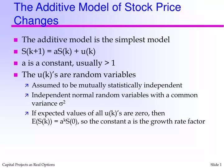
The Additive Model of Stock Price Changes. The additive model is the simplest model S(k+1) = aS(k) + u(k) a is a constant, usually > 1 The u(k)’s are random variables Assumed to be mutually statistically independent Independent normal random variables with a common variance 2

E N D
The Additive Model of Stock Price Changes • The additive model is the simplest model • S(k+1) = aS(k) + u(k) • a is a constant, usually > 1 • The u(k)’s are random variables • Assumed to be mutually statistically independent • Independent normal random variables with a common variance 2 • If expected values of all u(k)’s are zero, then E(S(k)) = akS(0), so the constant a is the growth rate factor
Criticisms of the Additive Model • Since the random term is a normally distributed random variable, the prices could go negative • The standard deviation should be proportional to the price
The Multiplicative Model • The multiplicative model has the form • S(k+1) = u(k)S(k) • u(k) is the relative (or percentage) change in S(k) • This relative change is S(k+1)/S(k), and independent of units (eg dollars, yen, etc.) • Taking the natural logarithms, we have the additive model • ln S(k+1) = ln S(k) + ln u(k) • define w(k) = ln u(k) • w(k)’s are normally distributed with expected value = and variance 2
Lognormal prices • Note that u(k) = ew(k) • The u(k)’s are lognormal random variables • Since ln S(k) = ln S(0) + • ln S(k) is lognormal also • E[ln S(k)] = ln S(0) + k • Var[ln S(k)] = k2 • Note: Empirical evidence supports this view
Estimating and • The value of w(k) = ln u(k) is the logarithm of the return on the stock, with a mean value and variance 2 • Typically, these parameters are estimated for a year. If the time period is a percentage of year p, then
The Mean • Suppose that w has expected value and variance 2 • Then the mean of the expected rate of increase is given by • Note that there is a “correction factor” related to the variance of the distribution. • As the variance increases, the lognormal distribution spreads out, but cannot go below zero, so the mean increases as a function of the variance
Random Walks • We define the additive process z by • This process is a random walk, and is a normal random variable with mean 0 and variance equal to 1
Wiener Process • A Wiener process is obtained by taking the limit of a random walk as t goes to 0 • In symbolic form, we have • A process z(t) is a Wiener process if • For any s<t the quantity z(t) – z(s) is a normal random variable with mean zero and variance t-s • For any 0<t1<t2<t3<t4, the random variables z(t2) – z(t1) and z(t4) – z(t3) are uncorrelated • z(t0) = 0 with probability 1
Wiener Process (Continued) • Intuitively, a continuous time version of a random walk • A generalized Wiener process has the form • where x(t) is a random variable for each t, z is a Wiener process, and a and b are constants • An Ito process is written • where z is a Wiener process
Stock prices and Wiener processes • The multiplicative model of stock prices ln S(k+1) – ln S(k) = w(k) may be written in continuous time as d ln S(t) = dt + dz where z is a standard Wiener process • dt may be interpreted as the mean value of the right hand side, and is proportional to dt • The standard deviation of the right hand side is times the standard deviation of dz, which is of the order of magnitude of dt • The continuous time model is a generalized Wiener process with solution ln S(t) = ln S(0) + t +z(t), so E[ln S(t)] = E[ln S(0)] + t
Lognormal prices • The continuous time solution is termed geometric Brownian motion, and is a lognormal process • The mean value must be adjusted, and is • If we define = + .52 • The standard deviation is given by
The Ito Process for Prices • We can express the random process for prices in terms of S(t) rather than in terms of its ln • This requires a correction using Ito’s lemma • Using = + .52 we obtain the standard Ito form for price dynamics
Summary of relations for Brownian motion • Suppose the geometric Brownian process S(t) is governed by • where z is a standard Wiener process. Let = + .52. Then S(t) is lognormal and
A Review of Financial Options • Options: Special contractual arrangements giving the owner the right to buy or sell an asset at a fixed price anytime on or before a given date. • Types of Options: • Stock options - traded on organized exchanges since 1973. • Currency, commodity and interest rate options. • Corporate securities - bonds, warrants and other convertibles. • Capital structure decisions - lender acquires company and shareholders obtain option to buy it back by paying off debt. • Capital-budgeting decisions - oil and mineral leases.
Characteristics of Options • Not bought for the usual benefits offered by other securities, i.e. interest and dividends. • Alternative to investing in a security. • Options' expected return is greater than the underlying security (and so is its risk). • Motivations for participating in option market • Speculate in an attempt to grab a quick buck. • Earn extra income on a security you already own. • Hedging mechanism for existing position.
What is an Option? • Listed options are contracts that give the holder the right (but not the obligation) to buy or sell a pre-specified security at a pre-specified price by a pre-specified date. • Call options give the owner the right to buy 100 shares of a specific stock at a specific price. • Put options give the owner the right to sell 100 shares of a specific stock at a specific price. • Calls and Puts are very distinct investments. • Calls are an expression of the buyer's optimism - you buy calls if you expect stock prices to rise. • Puts are bearish investments - you expect stock prices to fall.
Option Terminology • Option Buyer (Holder or Owner) - the individual who obtains the right to exercise. • Option Seller (Writer) - the individual who is obligated, if and when he or she is assigned an exercise notice, to perform according to the terms of the option contract. • Exercise (Strike) Price - For a call, the price per share at which the holder can purchase the underlying stock from the option writer; for a put, the price at which the holder can sell the underlying stock to the option writer. • Expiration Date -stock options expire on the Saturday following the third Friday of the expiration month; expirations are based on a 3-month calendar cycle. • Premium - price paid by the buyer to the writer of an option; set in the marketplace by investors' demand and supply.
Option Terminology (cont’d) • American and European Options - An American option may be exercised anytime up to the expiration date; a European option differs in that it can be exercised only on the expiration date. • "In-the-Money" Option - A call option is "in-the-money" whenever its exercise price is below the current stock price. Conversely, a put option is "in-the-money" whenever its exercise price is above the current stock price. Such options are said to have intrinsic value. • "Out-of-the-Money" Option - A call option is "out-of-the-money" whenever its exercise price is above the current stock price. Conversely, a put option is "out-of-the-money" whenever its exercise price is below the current stock price. Such options are said to have no intrinsic value.
Call Option - An Example Suppose Mr. Optimist holds a six month call option for 100 shares of Exxon common stock. It is a European call option and can be exercised at $150 per share. Now assume that the expiration date has arrived. What is the value of the Exxon call option on the expiration date? Answer: If Exxon is selling for $200 share, Mr. Optimist can exercise the option - purchasing 100 shares of Exxon at $150 per share - and then immediately sell the shares at $200. Mr. Optimist will have made $5,000 (100 shares x $50). Let St be the stock price on the exercise date, then Payoff on Expiration Date If St $150, then call option value = $0 If St > $150, then call option value = St - $150 Conversely, assume that Exxon is selling for $100 per share on the expiration date, If Mr. Optimist still holds the call option, he will throw it out.
A Graphical View of a Call Option Assumes options are in lots of 100
Put Option - An Example Suppose Ms. Pessimist feels quite certain that Exxon will fall from its current $160 share price. She buys a put. Her put contract gives her the right to sell 100 shares of Exxon at $150 six months from now. Now assume that the expiration date has arrived. What is the value of the Exxon put option on the expiration date? Answer: If Exxon is selling for $200 share, Ms. Pessimist will tear up the put option and throw it away - it is worthless. On the other hand, if Exxon is selling for $100 per share, Ms. Pessimist can purchase 100 shares of Exxon at $100 per share - and then immediately exercise her option to sell the shares at $150. Ms. Optimist will have made $5,000 (100 shares x $50). Value of the put option on the exercise date is $5000. Again, let St be the stock price on the exercise date, then Payoff on Expiration Date If St< $150, then call option value = $150 - St If St $150, then call option value = $0
Call and Put Option Quotes Mobil Oil Corporation Column 1 - Stock of Mobil Oil closed at $697/8 per share on the previous day (Monday, January 20). Column 2 & 3 - Indicates that Monday's closing price for an option maturing at the end of February with a striking price of $60 was $101/4. Because it is a 100-share contract, the cost of the contract is $1025. Columns 6, 7, & 8 - Quotes on puts; for example, a put maturing in February with an exercise price of $65 sells at $5/8.
Some Observations on Option Pricing • For a given exercise price, the premium steadily increases moving across time (from February to April). This occurs because of an option’s time value. • Time value of an option is that portion of an option's premium that represents what investors are willing to pay in hopes that the option will increase in value as the stock price increases. • Farther away from expiration, the greater a put or call option's time value will be. • For a given expiration date (reading down a column), a call's premium decreases, but a put's premium increases. • EX.: In February, the 60 call is "in-the-money" (has intrinsic value), the 75 call is "out-of-the-money" (has no intrinsic value). With the puts, just the opposite occurs.
Option Behavior vs. Stock Behavior • The value of the call increases with the value of the stock, while the value of the put decreases with value of the stock. • Unless the option is certain to be exercised, the absolute dollar change in the stock value is greater than the accompanying absolute dollar change in the option value. • The difference between the absolute dollar changes for the stock and for the options becomes smaller as the options move "out-of-the money" to "in-the-money". • The absolute percentage changes in the option prices are greater than the accompanying absolute percentage changes in the stock price. • The difference in the absolute percentage changes between the stock and the options again becomes smaller as the options move from being out-of-the money" to "in-the-money". Thus, out-of-the-money options are inherently more volatile.
Financial Options and Leverage • Major advantages of buying puts and calls are their speculative appeal in: • leveraging potential investment returns • limiting potential losses • reducing the required investment. • A Call Option Example: Let's say you are bullish on Mobil Oil stock that is currently priced at $40/share. You could: (1) Invest $4000 in 100 shares or (2) Invest only $400 to buy a Mobil June 40 call Let's compare and contrast the absolute dollar profits (losses) and percentage returns associated with different stock prices at the exercise date. 1. Stock rises to $50. 2. Stock Remains at $40. 3. Stock drops to $30.
How Options Affect Risks and Rewards Stock Price = $40 Call Option Premium = $4 Put Option Premium = $4 • Contrast gains between stock and call at $50 price: Need less capital to buy the option and participate $ for $ in stock’s appreciation. • The more leveraged the investment, the greater the risk that a large percentage of it will be lost. • Compared to stock ownership, dollar losses for calls and puts are limited.
What about a riskless return? • One strategy in the options market may offset another strategy, resulting in a riskless return. Example of an Offsetting Strategy: Suppose the stock price is currently $44. At the expiration date, the stock will either be $58 or $34. Consider the following: (1) Buy the stock; (2) Buy the put; and (3) Sell the call. Payoffs at expiration are:
What About Your Investment Capital? • Suppose you originally paid $44 for the stock, $7 for the put and received $1 for selling the call. • Because you paid out $50 and will receive $55 in one year, you have earned 10% ROR - the equilibrium rate of interest. Conversely, if the put sold for only $6 your initial investment would be $49. You would then have a non-equilibrium return of 12.2% ($55/$49 -1). • Put-Call Parity: It can be proved that, in order to prevent arbitrage, the prices at the time you take on your original position must conform to the following: Value of Stock + Value of Put - Value of Call = PV of Exercise Price $44 + $7 - $1 = $50 = $55/1.10 • This shows that the values of a put and call with the same exercise price and same expiration date are precisely related to each other.
Valuing Options - A Qualitative Look • Features of the Option Contract and Their Effects • Exercise Price (X) • Higher the exercise price, lower the value of the call option. • However, the value of a call option cannot be negative, no matter how high we set the exercise price. • As long as the is some probability that the price of the underlying asset will exceed the exercise price before the expiration date, the option will have value. • Time to Expiration (t) • Value of an American call option must be at least as great as the value of otherwise identical option with a shorter term to expiration. • Ex: Consider two options, one with a maturity of nine months and one with a maturity of six months. The nine-month option has the same rights as the 6-month call and also has an additional 3 months within which these rights can be exercised. (Not necessarily true with European options).
Qualitative Observations (cont’d) • Stock Price (S) • Higher the stock price, the more valuable the call option will be. • Relationship between stock price at exercise date and option value can be shown by the convex curve. • Variability of the Underlying Asset (2) • Greater the variability of the underlying asset, the more valuable the call option will be. • Ex.: Suppose just before call expires, stock price will be either $100 w/probability of 0.5 or $80 with probability of 0.5. What will be the value of a call with an exercise price of $110? • Now assume the stock price is much more variable; say $60 as the worst case and $120 as best case with same probabilities. Note that the expected value of the stock is the same ($90). However, now the call option has value because there is a one-half chance that the stock value will go to $120.
Qualitative Observations (cont’d) • Variability of the Underlying Asset (cont’d) • An Important Distinction Between Stocks and Options: • If investors in the marketplace are risk averse, a rise in the variability of the stock will decrease its market value. • However, holders of calls only are concerned about the positive tails of the probability distribution; as a consequence, a rise in the variability of the underlying stock increases the market value of the call. • The Interest Rate (r) • Buyers of calls do not pay the exercise price until they exercise the option, if they do so at all. • The delayed payment is more valuable when interest rates are high and less valuable when interest rates are low. • Value of a call is positively related to interest rates.
OPT - A Quantitative Approach • Ex.: Applying a Two-State Option Model • Suppose the market price of a stock is $50 and it will be either $60 or $40 at the end of the year. • Further suppose that there exists a call option for 100 shares of this stock with a one year expiration date and a $50 exercise price. Assume investors can borrow at 10%. • Let's examine two possible trading strategies: • 1. Buy a call on the stock. • 2. Buy 50 shares of the stock and borrow a duplicating amount. (Duplicating amount is the amount of borrowing necessary to make the future payoffs equivalent.
OPT - A Quantitative Approach (cont’d) • Future payoff structure of “buy a call” is duplicated by the strategy of “buy stock and borrow”. • Since the strategies are equivalent as far as market traders are concerned, the two strategies must have the same cost.
OPT - A Quantitative Approach (cont’d) The cost of purchasing 50 shares of stock while borrowing $1818 is: Buy 50 shares of stock 50 x $50 = $2500 Borrow $1818 at 10% -$1818 $ 682 • Because the call option gives the same return, the call must be priced at $682. This is the value of the call option in a market where no arbitrage profits exist. • Some Comments: • Note that we found the exact option value without even knowing the probability that the stock would go up or down! • The optimist and the pessimist would agree on the option value. How could that be? • The answer is that the current $50 stock price already balances the views of the optimists and pessimists - the option reflects that balance because its value depends on the stock price.
OPT and the Black-Scholes Model • Extension of the two-state model • B&S Model allows us to value a call in the real world by: • Determining the duplicating combination at any moment; • Valuing the option based on the duplicating strategy. • The Model: where S = Current stock price E = Exercise price of call r = Continuous risk-free rate of return (annualized) 2 = Variance (per year) of the continuous return on the stock t = Time (in years) to expiration date In addition, N(d) equals probability that a standardized, normally distributed, random variable will be less than or equal to d.
A Simple Example of Black-Scholes • Consider the Big Oil Company (BOC). On 10/4/97, BOC April 49 call option had a closing value of $4. The stock itself is selling at $50. On 10/4, the option had 199 days to expiration (maturity date = 4/21/98). The annual risk-free interest rate is 7 percent. From this we can determine the following variables: 1. Stock price, S, is $50. 2. Exercise price, E, is $49. 3. Risk-free rate, r, is 0.07. 4. Time to maturity in years, t, = 199/365. • Estimates of Variance may differ; but must obviously involve analysis of a series of past price movements for the stock. Let's assume variance of returns on BOC is estimated at 0.09/year.
Black-Scholes Example (cont’d) Step 1: Calculate d1 and d2 Step 2: Calculate N(d1) and N(d2) From a table of the cumulative probabilities of the standard normal distribution, we know that: N(d1) = N(0.3743) = 0.6459 N(d2) = N(0.1528) = 0.5607 Interpretation: N(d) is the cumulative probability of d. For example, N(d1) tells us that there is a 64.59 percent probability that a drawing from the standardized normal distribution will be below 0.3743.
Black-Scholes Example (cont’d) Step 3: Calculate the call option value (C) Note: The estimated price of $5.85 is greater than the actual price of $4; this implies the call option is underpriced!
Why is Black-Scholes So Attractive? • Four of the five necessary parameters are observable. • Investor's risk aversion does not affect value; formula can be used by anyone, regardless of willingness to bear risk. • It does not depend on the expected return of the stock. • Investors with different assessments of the stock's expected return will nevertheless agree on the call price. • As in the two-state example, the call depends on the stock price, and that price already balances investors' divergent views.