Download
1 / 18
180 likes | 252 Views
Spectro-imaging observations of H 3 + on Jupiter. Emmanuel Lellouch. Observatoire de Paris, France. H 3 + in planetary atmospheres. Discovered in 1988 in Jupiter’s auroral regions (Drossart et al. 1989) from its 2 2 emission

E N D
Spectro-imaging observations of H3+ on Jupiter Emmanuel Lellouch Observatoire de Paris, France
H3+ in planetary atmospheres • Discovered in 1988 in Jupiter’s auroral regions (Drossart et al. 1989) from its 22 emission • Since then, also discovered in Saturn and Uranus, and in Jupiter’s low latitude regions • General goals on the observations (esp. Jupiter) • Characterize the morphology and variability of the emission • Interpret the emission rates in terms of H3+ column density and temperature • Measure winds from Doppler shifts on H3+ emissions • Bands observed so far on Jupiter: 2, 22, 22 - 2 • H3+ traces and drives the energetics and dynamics of Giant Planets upper atmospheres (see Steve Miller’s talk)
Outline • Detection of the 3 2 - 2 band on Jupiter • The question of LTE and the multiplicity of H3+ « temperatures » • The spatial variations of the H3+ emission: do they trace variations in the H3+ column or « temperature »?
Spectro-imaging observations • Imaging FTS « BEAR » at Canada-France-Hawaii Telescope • Sept. 1999 & Oct. 2000 • 2 filters • 2.09 µm : 4760-4805 cm-1 • 2.12 µm : 4698-4752 cm-1 • 14 data cubes (2 spatial, 1 spectral dimension) sampling either the Northern or the Southern auroral region of Jupiter at various longitudes • See detailed report in Raynaud et al. Icarus, 171, 133 (2004)
Example of spectrum: 2.09 µm range 22 band
Example of spectrum: 2.12 µm range 22 and 32-2 bands H2 S1(1)
The two 32 - 2 lines Obs. freq. (cm-1) Calc. Freq. (cm-1) Assignment E’ (cm-1) (Neale et al. 1996) --------------------------------------------------------------------------------- 4721.79 4722.383 323 - 2 R(6,7) 7993.60 4749.66 4749.937 323 - 2 R(5,6) 7998.64 ---------------------------------------------------------------------------------
Temperature/column density determinations • Classical LTE formulation • This effectively assumes complete LTE (Trot = Tvib= Tkin) • Justified for rotational distribution (rad ~ 1000 sec, coll ~ 10-3 sec) • For vibrational distribution, rad ~ 10-2 sec non-LTE; however earlier studies (Y.H. Kim et al. 1992) have found that: • All the nv2 levels are underpopulated w.r.t. ground state • But their relative populations are close to LTE distribution : « quasi-LTE » distribution • Here: • 2.09 µm observations (2 2 lines only) determine Trot in v2 =2 level • 2.12 µm observations (including the 3 2 - 2 lines) determine Tvib (relative populations of v2 =2 and v2 = 3 levels)
Temperature results • Tvib • Trot Central meridian longitude In average, Trot = 1170+/-75 K > Tvib = 960 +/- 50 K underpopulation of v2 =3 relative to 2 = 2 with respect to LTE case
Trot and N (H3+) results • We get Trot (22) = 1170+/-75 K, and N = (4-8)x1010 cm-2 • Quite different from Lam et al. 1997: Trot (2) = 700-1000 K, and N ~ 1012 cm-2 • Interpretation: The 2 bands probe different levels in an atmosphere with strong positive temperature gradient Grodent et al. 2001
222 R(6,6) 2 Q(1,0) A non-LTE H3+ model (Melin et al. 2005) • Based on detailed balance calculations (Oka and Epp 2004) and a physical (temperature,density) model of Jupiter’s upper atmosphere • Calculate line production profile in atmosphere and compare with LTE situation • Results: • The 22 band probes higher and hotter atmospheric levels than 2 • Non-LTE effects are minor for 2 but much more significant for 2 2 lines • Thus, using 2 2 lines leads to too low a column density Melin et al. 2005
222 R(6,6) 323- 2R(5,6) Melin et al. 2005 Trot vs. Tvib • We find Trot = 1170+/-75 K > Tvib = 960 +/- 50 K, i.e. an underpopulation of v2 =3 relative to v2 =2 with respect to LTE case • Interpretation: • non-LTE effects are even more significant for 32 - 2 (and higher overtones) than for 22 lines the temperaturedetermined by assuming QLTE for v2 =2 and v2 =3 underestimates Tkin Melin et al. 2005
Beyond the QLTE hypothesis • Main conclusion: non-LTE effects are severe • May induce large errors in T and especially N (H3+) determined from overtone and hot bands (up to ~2 orders of magnitude underestimate for N (H3+) !) • Future studies: rather than « temperature/column density retrievals », better to perform forward modelling , i.e. test Tkin(z), n(H3+) profiles directly against data
Spatial distribution of emissions: H2 vs. H3+ H3+ 222 R(7,7): 4732 cm-1 H2 S1(1): 4712 cm-1 H3+ 323- 2R(6,7): 4722 cm-1 « Hot spot » near = 70°N, LIII = 160°
Variations in H3+ emission rates : variations in temperature or column density ? 1-5 = five bins of increasing emission (5 = « hot spot » near LIII = 160°) • Except in « hot spot », emission variations mostly due to variations in N(H3+) • Confirmed by search for correlations between intensities/temperatures/columns on individual pixels
Emission variations are mostly due to variations in N(H3+) • In agreement with Stallard et al. 2002 • Little or no temperature variations: thermostatic effect from H3+ • H3+ cooling dominant above homopause • e.g. T(0.01 µbar) ~1300 K. Would be 4800 K if no H3+ cooling (Grodent et al. 2001) • Large variations of input energy radiated by modest increases of temperature • E.g. « diffuse » and « discrete » aurora (differing by amount of hard electron precipitation) have similar (within ~100 K) temperatures • Exception: the « hot spot », actually hotter than other regions by ~250 K
Conclusions • We have detected the 32 - 2 band of H3+ on Jupiter • Our temperature/column density determinations differ with those obtained from other bands. This can be understood from: • Strong non-LTE effects on combination and overtone bands • The temperature profile in Jupiter’s auroral ionosphere • Spatial variations in the H3+ emission generally trace variations in H3+ columns and not in temperature • The increased temperature in the « hot spot » (also visible at other wavelengths but NOT in H2 emission) remains a mystery
The H3+ Northern auroral « hot spot » • Located at ~70°N, LIII ~ 160 • Has Tvib ~ 250 K warmer than other regions • Region peculiar at other : • Thermal IR emission of several hydrocarbons • Far UV (footprint of polar cusp) • X-ray emission • But not in H2 S1(1) ! • Origin? • Impact of very energetic (> 100 keV) electron (cf origin of FUV features)? • Would rather produce ‘deep’ (cold) H3+ • Increased vertical mixing due to increased precipitation, resulting in elevated homopause? • Increased CH4 reduces the deep cold H3+ component increase of mean H3+ temperature • But is it consistent with increase of H3+ emission? • Why not seen in H2 ?