Download

1 / 33
350 likes | 512 Views
CS 425/ECE 428/CSE 424 Distributed Systems (Fall 2009). Lecture 16 Distributed Graph (Routing) Algorithms Source: (1) Book “Distributed Systems: an Algorithmic Approach”, S. Gosh, Chapter 10.1-10.2.3 “Graph Algorithms” and (2) Chapter 3 in our textbook Klara Nahrstedt. Acknowledgement.

E N D
CS 425/ECE 428/CSE 424Distributed Systems (Fall 2009) Lecture 16 Distributed Graph (Routing) Algorithms Source: (1) Book “Distributed Systems: an Algorithmic Approach”, S. Gosh, Chapter 10.1-10.2.3 “Graph Algorithms” and (2) Chapter 3 in our textbook Klara Nahrstedt
Acknowledgement • The slides during this semester are based on ideas and material from the following sources: • Slides prepared by Professors M. Harandi, J. Hou, I. Gupta, N. Vaidya, Y-Ch. Hu, S. Mitra. • Slides from Professor S. Gosh’s course at University o Iowa.
Administrative • Homework 2 is graded and solutions are posted • Homework 3 is posted • Deadline: October 29, Thursday, 2 pm in class • Midterm is graded and solutions are posted • Midterm Re-grading Period by Instructor • October 27, 3:15-4pm • October 29, 3:15-4pm • No instructor office hours during the week of October 19-24 • (Instructor is at ACM International Conference on Multimedia 2009 in Beijing, China)
Administrative • MP2 posted October 5, 2009, on the course website, • Deadline November 6 (Friday) • Demonstrations , 4-6pm, 11/6/2009 • You will need to lease one Android/Google Developers Phone per person from the CS department (see lease instructions)!! • Start early on this MP2 • Update groups as soon as possible and let TA know by email so that she can work with TSG to update group svn • Tutorial for MP2 planned for October 28 evening if students send questions to TA by October 25. Send requests what you would like to hear in the tutorial. • During October 15-25, Thadpong Pongthawornkamol (tpongth2@illinois.edu) will held office hours and respond to MP2 questions for Ying Huang (Ying is going to the IEEE MASS 2009 conference in China)
Administrative • MP3 proposal instructions • MP3 proposal is posted • You will need to submit a proposal for MP3 on top of your MP2 before you start MP3 on November 9, 2009 • Deadline for Proposal: October 25, 2009, email proposal to TA • At least one representative of each group meets with instructor or TA during October 26-28 during their office hours ) watch for extended office hours during these days. • Instructor office hours: October 28 times 8:30-10am
Administrative • To get Google Developers Phone, you need a Lease Form • Fill out the lease form; bring the lease form to Rick van Hook/Paula Welch and pick up the phone from 1330 SC • Lease Phones: phones will be ready to pick up starting October 20, 9-4pm from room 1330 SC (purchasing , receiving and inventory control office) • Return Phones: phones need to be returned during December 14-18, 9-4pm in 1330 SC
Distributed Graph Algorithms • why graph algorithms ? It is not a “graph theory” course! • many problems in networks can be modeled as graph problems • the topology of a distributed system is a graph • routing table computation uses the shortest path algorithm • efficient broadcasting uses a spanning tree • Max flow algorithm determines the maximum flow between a pair of nodes in a graph.
Routing • Shortest path routing • Distance vector routing • Link state routing • Routing in sensor networks • Routing in peer-to-peer networks • Geographic routing
Plan for Today • Routing algorithms • Chandy-Misra (distributed Bellman-Ford) • Distance vector • Link state • Interval routing
PCs,routers, switches… =nodes links= edges The Internet (Internet Mapping Project, color coded by ISPs)
Message Layers Application Messages (UDP) or Streams (TCP) Transport UDP or TCP packets Internet IP datagrams Internet Routing Algorithms Network interface Network-specific frames Underlying network Internet 5-Layer Model
Intra-AS Routing Revisited Source: http://www.cisco.com
Internet Routing • intra-AS routing • Open Shortest Path First(OSPF) • a link state protocol • (RFC 2328(1998) forIPv4, updated in RFC 5340(2008) • inter-AS routing • Border Gateway Protocol (BGP) • path vector protocol • makes routing decisions based on path, network policies and/or rule sets
Routing: shortest path • most shortest path algorithms are adaptations of the classic Bellman- Ford algorithm. Computes shortest path if there are no cycle of negative weight • Let D(j) = shortest distance of j from initiator 0. Thus D(0) = 0 The edge weights w(j,k) can represent latency or distance or some other appropriate parameter
Shortest path revisiting Bellman Ford : basic idea Consider a static topology process 0 sends w(0,i), 0 to neighbor i {program for pi} upon receiving message (dist, k) if dist < Di then if parent ≠ k then parent := k fi; Di := dist; send (Di + w(i,j), i) to each neighbor j ≠ parent; if dist ≥ Dithen do nothing Current distance Compute the shortest Distance to all nodes From an initiator node
Chandy&Misra’s Shortest Path (assumes static topology) /* D initialized to ∞, parent = i; deficit = 0, each message has format (distance, sender) */ {for process 0} Process 0 sends w(0,i), 0 to neighbor i, deficit=|N(0)| ; /*N(0) set of successors of node 0; N(i) set of neighbors of node i */ do deficit > 0 & ack, deficit:= deficit – 1 od; (deficit = 0 signals termination) {for process i>0} domessage(S,k) & S<D /* S value of distance received through message, D shortest distance between node 0 and i */ if parent ≠ k & deficit > 0 send ack to parent fi; parent:= k; D:=S; send(D + w(i,j),i) to each neighbor j ≠ parent; deficit:=deficit+|N(i)|; message(S,k) & S≥D send ack to sender; ack deficit:=deficit–1; deficit=0 & parent ≠ I send ack to parent; od
Shortest Path • an important issue is: how well do such algorithms perform when the topology changes? No real network is static! • let us examine distance vector routing and link state routing - adaptations of the shortest path algorithm
Internet Routing Algorithms • Programmed in the network layer • determine the “next hop”, given the destination IP address, • thus determine the route for each packet as it travels through the net, • dynamically update routing information to reflect failures, changes and congestion. • Two approaches: • link-state (e.g., OSPF) • Every node knows status of each “link” in the network • distance-vector (e.g., RIP) • Every node knows the next-hop for each possible destination LAN Information maintained as a table Tables updated either • Proactively – periodically, or • Reactively – when a neighbor/some link status changes
Distance Vector Routing Distance Vector D for each node i contains N elements Dj[0], Dj[1], Dj[2]… Initialize to ∞ {Dj[i] is distance from node j to node i.} - Each node j periodically sends its distance vector to its immediate neighbors. - Every neighbor i of j, after receiving the broadcasts from its neighbors, updates its distance vector as follows: For all k≠i: Di[k]=minj(w[i,j] + Dj[k]) Used in IGRP etc • Dj[k]=3 means j thinks k is 3 hops away
Distance Vector Routing Protocol • Also termed as distributed Bellman-Ford algorithm or Ford-Fulkerson algorithm, included in RIP (routing information protocol), AppleTalk, and Cisco routers. • Each node/router maintains a table indexed by each destination node. Entry gives the best known distance to destination and which link to use for forwarding. • Once every T seconds each router sends to each neighbor its own entire table (proactive)
Routers 1 B 2 A C 4 3 5 E D 6 Hosts or LANs To Link Cost A 1 1 C 2 1 D 4 2 E 4 1 B local Distance Vector Routing Routing Table for A Routing Table for B To Link Cost B 1 1 C 1 2 D 3 1 E 1 2 A local To Link Cost A 2 2 B 2 1 D 5 2 E 5 1 C local Link number (all links have cost=1) Routing Table for C
DVR • What may go wrong? • What if links fail?
Counting to Infinity node 1 thinks D1[3] = 2 node 2 thinks D2[3] = D1[3]+1 = 3 node 1 thinks D1[3] = D2[3]+1 = 4 and so on; it will take forever for the distances to stabilize one remedy is the split horizon method that prevents 1 from sending the advertisement about D1[3] to 2 since its first hop is node 2 Observe what can happen when the link (2,3) fails. For all k≠ i: Di[k] = mink(w[i,j] + Dj[k] ) Suitable for smaller networks. Larger volume of data is disseminated, but to its immediate neighbors only Poor convergence property
Link State Routing Each node i periodically broadcasts the weights of all edges (i,j) incident on it (this is the link state) to all its neighbors. The mechanism for dissemination is flooding This helps each node eventually compute the topology of the network, and independently determine the shortest path to any destination node using some standard graph algorithm like Dijkstra’s Smaller volume data disseminated over the entire network - Used in OSPF
Link State Execution Link state (list of neighbor nodes, and their weights)
Link State Routing • each link state packet has a sequence number seqthat determines the order in which the packets were generated • what’s the problem ? • need unbounded counters • when a node crashes, all packets stored in it are lost • after it is repaired, new packets start with seq= 0, so these new packets may be discarded in favor of the old packets! – problem resolved using TTL
Link State Routing Protocol • Each router must • Discover its neighbors and learn their network addresses • When a router is booted, it learns who its neighbors are by sending a special Hello packet on each point-to-point link. • The router on the other end sends back a reply. • Measure the delay or cost to each of its neighbors • A router sends a special Echo packet over the link that the other end sends back immediately. By measuring the round-trip time, the sending router gets a reasonable delay estimate. • Construct a packet telling all it has just learned. • Broadcast this packet
Link State Routing (Example) • A router broadcasts a link-state-advertisement (LSA) packet after booting, as well as periodically (or upon topology change). Packet forwarded only once, TTL-restricted • Initial TTL is very high.
Link State Routing Protocol • Broadcast the LSA packet to all other routers in the subnet. • Each packet contains a sequence number that is incremented for each new LSA packet sent. • Each router keeps track of all the (source router, sequence) pairs it sees. When a new LSA packet comes in, it is checked against the pairs. If the received packet is new, it is forwarded on all the links except the one it arrived on. • The age of each packet is included and is decremented once per time unit. When the age hits zero, the information is discarded. Initial age = very high • For routing a packet, since the source knows the entire network graph, it simply computes the shortest path (actual sequence of nodes) locally using the Dijkstra’s algorithm.
Summary • Graph algorithms • Standard routing algorithms like shortest path, distance vector • The final outcome of these protocols is set of routing tables (on for each node) • Conventional routing tables have space complexity of O(N) • Need for adaptability to changing topologies