Download
1 / 30
300 likes | 396 Views
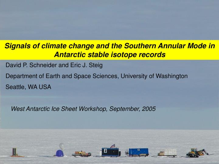
Signals of climate change and the Southern Annular Mode in Antarctic stable isotope records. David P. Schneider and Eric J. Steig Department of Earth and Space Sciences, University of Washington Seattle, WA USA West Antarctic Ice Sheet Workshop, September, 2005.

E N D
Signals of climate change and the Southern Annular Mode in Antarctic stable isotope records David P. Schneider and Eric J. Steig Department of Earth and Space Sciences, University of Washington Seattle, WA USA West Antarctic Ice Sheet Workshop, September, 2005
…and in climate models. David P. Schneider and Eric J. Steig Department of Earth and Space Sciences, University of Washington Seattle, WA USA West Antarctic Ice Sheet Workshop, September, 2005
Outline Objective: A constrained range of possible Antarctic climate histories using data-model comparisons. 1) Temperature histories 2) Spatial variability of Southern Annular Mode (SAM) signal in δ18O and δD 3) What to do next
1) Temperature histories – Instrumental Record Continental stations with good T records
1) Temperature histories – Instrumental Record Continental stations with good T records T record average and Marshall (2003) SAM index r(A8, SAM) = -0.51
1) Temperature histories – Ice Core Records For calibration: Use multiple linear regression or combine cores into a single record, ice
1) Temperature histories – Ice Core Records, calibration with instrumental A8 Old method: multiple linear regression – important caveat about variance
1) Temperature histories – Ice Core Records, new calibration with instrumental A8 We use the stack of ice cores to reconstruct the stack of Antarctic temperature anomalies, A8. Reconstruction, R(t), is obtained as: Scale the standard deviation Scale the mean r (A8, ice) = 0.58 [Annual resolution 1961-1999] (similar to r2 of 30-40% found in Global Network of Isotopes in Precipitation (GNIP); Rozanski et al., 1992)
1) Temperature histories – Ice core based reconstruction Reconstruction Southern Hemisphere (SH) mean T observed A8
1) Temperature histories – Ice core based reconstruction compared with instrumental record and models Trend uncertainty is high in Antarctic records due to high variability! Linear trends (°C per 100 yrs w/ 95% confidence intervals) in the SH mean, Antarctic reconstruction, and NCAR climate model Time period SH meanAntarctic recon. CCSM3 Antarctic CCSM3 SH mean 1856-1999 0.44 ± .09 0.21 ± .26 *0.75 ± .14 *0.56 ± .07 1856-1975 0.32 ± .10 0.21 ± .35 *0.60 ± .25*0.47 ± .12 1976-1999 1.40 ± .59 **-2.2 ± 3.8 1.70 ± 3.5 1.20 ± .86 *Data begin in 1880; **A8 instrumental record used
1) Temperature histories – Last 50 years, instrumental data and model NCAR MODEL’S ANTARCTIC CONTINENT MEAN A8, STATION DATA MEAN SOUTHERN HEMISPHERE MEAN
1) Temperature histories – Global perspective from ice cores??
1) Temperature histories – Summary Results and key issues • Can reconstruct interannual “Antarctic temperature” using ITASE, Law Dome, etc. records with an r2 of 0.36 • Reconstruction indicates Antarctic change less than that observed in SH mean instrumental record • Latest NCAR model indicates polar amplification in the Antarctic • Ice core reconstruction agrees better than models with instrumental data showing recent cooling trend over Antarctica • Could reconstruct interdecadal “Global temperature” using Antarctic + Greenland cores with an r2 of 0.40 • The wiggles match, but do we trust the trends?
Isotopes = more than “temperature” Climate models with isotopic tracers can tell us what else. Some views from isotope GCMs: “The temperature dependence of precipitation facilitates an association between temperature and δ in proxy records. The small magnitudes of the correlation coefficients suggest that direct interpretation of proxy records such as temperature or precipitation should proceed under utmost scrutiny because reconstruction is far more complex than the problem of local regression…” [Noone and Simmonds, 2002] “The isotope variability simulated in this experiment from the interaction of several aspects of climate.” “Except for a modest relationship to temperature, isotopic variability over continents is not strongly coupled to an individual climate forcing factor. Instead, it probably reflects a shifting combination of factors or factors we have not considered.” [Cole and others, 1999]
2) Spatial variability of Southern Annular Mode signal in δ18O and δD
2) Spatial variability of Southern Annular Mode signal in δ18O and δD Using a climate model with isotopic code [Noone and Simmonds, 2002]. The signal of positive SAM depicted: - .2 - .6 ‰
2) Spatial variability of Southern Annular Mode signal in δ18O and δD Reminder of ITASE ice coring sites – site names and accumulation rates
2) Spatial variability of Southern Annular Mode signal in δ18O and δD Use ITASE cores. How does the ice core signal compare with T anomalies and model δ anomalies associated with SAM? Results of compositing analysis:
2) Spatial variability of Southern Annular Mode signal in δ18O and δD Results of compositing analysis are interesting: • We see consistent associations of δ anomalies with “Mode 1” indices (A8 SAM, etc) • These associations are only found at the relatively low accumulation sites (1999 and 2000 ITASE traverse areas; NOT high accumulation 2001 traverse area towards Pine Island - Thawaties) • In the 1999 and 2000 traverse areas, on the basis of just local temperature anomalies, you would expect stronger associations with “Mode 2” indices • Suggests that SAM-related variability dominates the isotope signal, but only in a certain area • Why?
2) Spatial variability of Southern Annular Mode signal in δ18O and δD Results of compositing analysis are interesting: • If a real feature of the climate system – look to accumulation rate records and models ITASE accumulation record study of Kaspari et al. (in press) has found: + Association of accumulation in 2001 traverse area with cyclonic activity in Amundsen, Bellingshausen and Ross seas (near coast) and a slight recent increase + Accumulation record in 1999-2000 traverse area consistent with moisture source farther to the north and a slight recent decrease
2) Spatial variability of Southern Annular Mode signal in δ18O and δD Results of compositing analysis are interesting: • If a real feature of the climate system – look to accumulation rate records and models Isotope GCM study of isotopic signature of SAM has found (Noone and Simmonds 2002): Positive SAM means: *Number and depth of cyclones near coast is increased *Moisture source nearer to the coast has enriching influence on inland precipitation High accumulation; Moisture source near coast
2) Spatial variability of Southern Annular Mode signal in δ18O and δD Results of compositing analysis are interesting: • If a real feature of the climate system – look to accumulation rate records and models Isotope GCM study of isotopic signature of SAM has found (Noone and Simmonds 2002): Positive SAM means: *Number and depth of cyclones near coast is increased *Moisture source nearer to the coast has enriching influence on inland precipitation *Moisture from farther north travels less direct path through zone of increased rain out; more distillation means more depletion of inland precip. (this dominates); cyclones travel inland easier High accumulation; Moisture source near coast Low accumulation; relies on moisture source more distant
3) What to do next • What’s next: • More data – model comparisons are needed to constrain climate reconstructions and interpretation of both isotope records and model output. • If we (Noone and others) can reasonably forward model the physics and climate processes involved in δanomalies on the WAIS, we can work towards an Antarctic climate reconstruction (inverse problem) using the observed (ice core) δmeasurements directly. Then we can do this globally using Antarctic + Greenland + other records. Apply to many new records (ITASE II, IPICS, etc.) and timescales of interest. • Result: Better climate reconstructions, better models. Need to use statistics + physics.
The end THANK YOU FOR YOUR ATTENTION
The end THANK YOU FOR YOUR ATTENTION
Part 1: Temperature Reconstruction Regressions onto A8
A 200-year temperature reconstruction We use the stack of ice cores to reconstruct the stack of Antarctic temperature anomalies, A8. Reconstruction, R(t), is obtained as: Scale the standard deviation Scale the mean r (A8, ice) = 0.58 [Annual resolution 1961-1999] (similar to r2 of 30-40% found in Global Isotopes in Precipitation Network (GNIP); Rozanski et al., 1992)
Outline PART 1 Problems / context PART 2 What is Antarctic climate variability like? PART 3 What aspects of the climate system are sampled by stable isotope ratios in ice cores? PART 4 A 200-year Antarctic climate reconstruction PART 5 Conclusions & Outlook
Conclusions & Outlook • Many types of data have been examined; fit within consistent framework • SAM imparts a high variability on temperature and stable isotope anomalies across the Antarctic continent; should be a priority for reconstruction • Long-term Antarctic temperature change appears to be small (and not statistically significant), but nonetheless there is a significant correlation of Antarctic temperature reconstruction with the SH mean • Climate models generally depict larger and more significant long-term climate change 1800s-present than ice cores • Some difference between SH temperature trend and Antarctic temperature trend can be attributed to SAM trend since 1970s; SAM surface signature weak in models
Conclusions & Outlook • Temporal δ-T slope different than spatial slope because of SAM? • Can SAM effect be separated from temperature effect? • Can isotope GCMs be used to “reconstruct” climate from isotope observations? • Spatially resolved reconstructions • Longer, lower frequency reconstructions with more proxies (2000 year time scale)? • Application to LGM and last 8 glacial cycles?