Download
1 / 37
370 likes | 642 Views
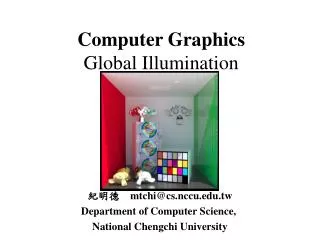
Global Illumination. Jian Huang, CS 594, Fall 2002 This set of slides reference text book and the course note of Dutre et. al on SIGGRAPH 2001. Looking Back. Ray-tracing and radiosity both computes global illumination Is there a more general methodology? It’s a game of light transport.

E N D
Global Illumination Jian Huang, CS 594, Fall 2002 This set of slides reference text book and the course note of Dutre et. al on SIGGRAPH 2001
Looking Back • Ray-tracing and radiosity both computes global illumination • Is there a more general methodology? • It’s a game of light transport.
Radiance • Radiance (L): for a point in 3D space, L is the light flux per unit projected area per unit solid angle, measured in W/(sr-m2) • sr – steradian: unit of solid angle • A cone that covers r2 area on the radius-r hemisphere • A total of 2p sr on a hemisphere W. • power density/solid angel • The fundamental radiometric quantity
Irradiance and Radiosity • Irradiance (E) • Integration of incoming radiance over all directions, measured in W/m2 • Incident radiant power (Watt) on per unit projected surface area • Radiance distribution is generally discontinuous, irradiance distribution is generally continuous, due to the integration • ‘shooting’, distribute radiance from a surface • ‘gathering’, integrating irradiance and accumulate light flux on surface • Radiosity (B) is • Exitant radiant power (Watt) on per unit projected surface area, measured in W/m2 as well
Path Notation • A non-mathematical way to categorize the behavior of global illumination algorithm • Diffuse to diffuse transfer • Specular to diffuse transfer • Diffuse to specular transfer • Specular to specular transfer • Heckbert’s string notation (1990): as light ray travels from source (L) to eye (E): • LDDE, LDSE+LDDE, LSSE+LDSE, LSDE, LSSDE
BRDF • Materials interact with light in different ways, and different materials have different appearances given the same lighting conditions. • The reflectance properties of a surface are described by a reflectance function, which models the interaction of light reflecting at a surface. • The bi-directional reflectance distribution function (BRDF) is the most general expression of reflectance of a material • The BRDF is defined as the ratio between differential radiance reflected in an exitant direction, and incident irradiance through a differential solid angle
BRDF • The geometry of BRDF
BRDF properties • Positive, and variable in regard to wave-length • Reciprocity: the value of the BRDF will remain unchanged if the incident and exitant directions are interchanged. • Generally, the BRDF is anisotropic. • BRDF behaves as a linear function with respect to all incident directions.
BRDF Examples • Diffuse surface (Lambertian) • Perfect specular surface • BRDF is non-zero in only one exitant direction • Glossy surfaces (non ideally specular) • Difficult to model analytically • Transparent surfaces • Need to model the full sphere (hemi-sphere is not enough) • BRDF is not usually enough, need BSSRDF (bi-directional sub-surface scattering reflectance distribution function) • The transparent side can be diffuse, specular or glossy
Reflectance • 3 forms
The Rendering Equation • Proposed by Jim Kajiya in his SIGGRAPH’1986 paper • Light transport equation in a general form • Describes not only diffuse surfaces, but also ones with complex reflective properties • Goal of computer graphics: solution of the rendering equation! • Looks simple and natural, but really is too complex to be solved exactly; various techniques to nd approximate solutions are used
The Rendering Equation • I(x,x’) = intensity passing from x’ to x • g(x,x’) = geometry term (1, or 1/r2, if x visible from x’, 0 otherwise) • e(x,x’) = intensity emitted from x’ in the direction of x • r(x,x’,x’’) = scattering term for x’ (fraction of intensity arriving at x’ from the direction of x’’ scattered in the direction of x) • S = union of all surfaces
Linear Operator • Define a linear operator, M. • The rendering equation: • How to solve it?
Neumann Series Solution • Start with an initial guess I0 • Compute a better solution • Computer an even better solution • Then, • In practice one needs to truncate it somewhere
Examples • No shading/illumination, just draw surfaces as emitting themselves: • Direct illumination, no shadows: • Direct illumination with shadows:
Implications • How successful is a global illumination algorithm? • The first term is simple, just visibility • How an algorithm handles the remaining terms and the recursion? • How does it handle the combinations of diffuse and specular reflectivity • The rendering equation is a view-independent statement of the problem • How are the radiosity algorithm and the ray-tracing algorithm?
Monte Carlo Techniques in Global Illumination • Monte Carlo is a general class of estimation method based on statistical sampling • The most famous example: to estimate p • Monte Carlo techniques are commonly used to solve integrals with no analytical or numerical solution • The rendering equation has one such integral
Basic Monte Carlo Integration • Suppose we want to numerically integrate a function over an integration domain D (of dimension d), i.e., we want to compute the value of the integral I: • Common deterministic approach: construct a number of sample points, and use the function values at those points to compute an estimate of I. • Monte Carlo integration basically uses the same approach, but uses a stochastic process to generate the sample points. And would like to generate N sample points distributed uniformlyover D.
Basic Monte Carlo Integration • The mean of the evaluated function values at each randomly generated sample point multiplied by the area of the integration domain, provides an unbiased estimator for I: • Monte Carlo methods provides an un-biased estimator • The variance reduces as N increases • Usually, given the same N, deterministic approach produces less error than Monte Carlo methods
When to Use Monte Carlo? • High dimension integration – the sample points needed in deterministic approach exponential increase • Complex integrand: practically can’t tell the error bound for deterministic approaches • Monte Carlo is always un-biased, and for rendering purpose, it converts errors into noise!!
Two Types of Monte Carlo • Monte Carlo integration methods can roughly be subdivided in two categories: • those that have no information about the function to be integrated: ‘blind Monte Carlo’ • those that do have some kind of information available about the function: ‘informed Monte Carlo’ • Intuitively, one expects that informed Monte Carlo methods to produce more accurate results as opposed to blind Monte Carlo methods. • The basic Monte Carlo integration is a blind Monte Carlo method
Importance Sampling • An informed Monte Carlo • Importance sampling uses a non-uniform probability function, pdf(x), for generating samples. • By choosing the probability function pdf(x) wisely on the basis of some knowledge of the function to be integrated, we can often reduce the variance • Can prove: if can get the pdf(x) to match the exact shape of the function to be integrated, f(x), the variance of the integration estimation is 0. • Practically, can use a sample table to generate a ‘good’ pdf. • Intuitively, want to send more rays into the more detailed areas in space
Stratified Sampling • Importance sampling (probability) using a limited number of samples, which is the case for graphics rendering, does not have a guarantee. • Stratified sampling address this further: the basic idea of stratified sampling is to split up the integration domain in m disjunct subdomains (also called strata), and evaluate the integral in each of the subdomains separately with one or more samples. • More precisely:
More On Ray-Tracing • Already discussed recursive ray-tracing! • Improvements to ray-tracing! • Area sampling variations to address aliasing • Cone tracing (only talk about this) • Beam tracing • Pencil tracing • Distributed ray-tracing!
Cone Tracing (1984) • Generalize linear rays into cones • One cone is fired from eye into each pixel • Have a wide angle to encompass the pixel • The cone is intersected with objects in its path • Reflection and refraction are modeled as spherical mirrors and lenses • Use the curvature of the object intersecting that cone • Broaden the reflected and refracted cones to simulate further scattering • Shadow: proportion of the shadow cone that remains un-blocked
Distributed Ray-Tracing • Another way to address aliasing • By Cook, Porter, and Carpenter in 1984. • A stochastic approach to supersampling that trades objectionable aliasing artifacts for the less offensive artifacts of noise • ‘Distributed’: rays are stochastically distributed to sample the quantities • This method was covered during our recursive ray tracing lecture as extension to correct aliasing
Sampling Other Dimensions • Other than stochastic spatial sampling for anti-aliasing, can sample in other dimensions • Motion blur (distribute rays in time) • Depth of field (distribute rays over the area of the camera lens) • Rough surfaces: blurred specular reflections and translucent refraction (distribute rays according to specular reflection and transmission functions) • Soft shadow: distribute shadow feeler rays over the solid angle span by the area light source • In all cases, use stochastic sampling to perturb rays
Path Tracing • Devised by Kajiya in 1986 • An efficient variation of distributed ray tracing • At each intersection, either fire a refraction ray or a reflection ray (not both!!) • This decision is guided by the desired distribution of the different kinds of rays for each pixel • Don’t have a binary ray-tree for each initial ray • It is really a Monte Carlo method ! Need to use a quite large N. (Kajiya used 40 rays per pixel) • Unlike ray-tracing, path tracing traces diffuse rays as well as specular rays
Path • Global illumination: generate all paths of light transport that interact among different surfaces and compute an integration to solve the rendering equation • Direct paths: length = 1, direct illumination • Indirect paths: length > 1
Indirect paths - surface sampling • Simple generator (path length = 2): • select point on light source • select random point on surfaces • per path: • 2 visibility checks
Indirect paths - source shooting • “shoot” ray from light source, find hit location • connect hit point to receiver • per path: • 1 ray intersection • 1 visibility check
Indirect paths - receiver gathering • “shoot” ray from receiver point, find hit location • connect hit point to random point on light source • per path: • 1 ray intersection • 1 visibility check
Indirect paths • Same principles apply to paths of length > 2 • generate multiple surface points • generate multiple bounces from light sources and connect to receiver • generate multiple bounces from receiver and connect to light sources • • Estimator and noise characteristics change with path generator
Complex path generators • Bi-directional ray tracing • shoot a path from light source • shoot a path from receiver • connect end points • Combine all paths and weigh them
Bidirectional ray tracing • Parameters • eye path length = 0: shooting from source • light path length = 0: gathering at receiver • When useful? • Light sources difficult to reach • Specific brdf evaluations (e.g., caustics)
Classic ray tracing? • Classic ray tracing: • shoot shadow-rays (direct illumination) • shoot perfect specular rays only for indirect • ignores many paths • does not solve the rendering equation