Download
1 / 21
210 likes | 324 Views
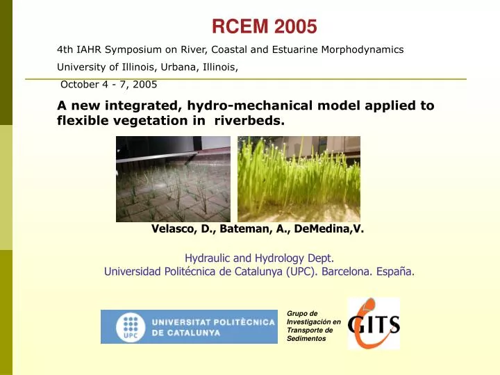
RCEM 2005 4th IAHR Symposium on River, Coastal and Estuarine Morphodynamics University of Illinois, Urbana, Illinois, October 4 - 7, 2005 A new integrated, hydro-mechanical model applied to flexible vegetation in riverbeds. Velasco, D., Bateman, A., DeMedina,V.

E N D
RCEM 2005 4th IAHR Symposium on River, Coastal and Estuarine Morphodynamics University of Illinois, Urbana, Illinois, October 4 - 7, 2005 A new integrated, hydro-mechanical model applied to flexible vegetation in riverbeds. Velasco, D., Bateman, A., DeMedina,V. Hydraulic and Hydrology Dept.Universidad Politécnica de Catalunya (UPC). Barcelona. España. Grupo de Investigación en Transporte de Sedimentos
Background • Kutija V., Hong (1996), Erduran, K.S., Kutija V (2003). • Flexible cylinders (cantilever deflection equation) • Eddy viscosity approach and mixing lenght theory • Discretization of vertical axis Z to apply an Unsteady Reynolds-x equation → converge to a steady solution • López,F., García,M.H. (2001), Fischer-Antze (2001) • 3D turbulent κ-εmodel • Rigid, vertical cylinders • Cui,J.,Neary V.S.(2002), Choi,S.,Kang,H.(2004) • 3D turbulent RANS and LES model • Rigid, vertical cylinders Variation of drag coeficients Cd as a function of Re number is never included. Incomplete Calibration (flexible vegetation flume flume data never used)
OBJECTIVES of the present work . 1) Creation of QUICKVEGMODEL, an integrated finite differencies model to calculate vertical velocity profile for vegetated channels, which includes a subroutine for flexible plant deformation. Input data is required for : a) vegetation properties: Plant geometry and Stiffness modulus (E) b) Hydraulic conditions: Drag Coeficients (Cd) 2) Verification of the “Large Deformation” model for plants Strain –stress tests in laboratory for different stems 3) Adjustment of QUICKVEGMODELparameters (calibration) using experimental data
1.) Description of QUICKVEGMODEL Vertical Integration of Reynolds equation between coordinates z=h and z Eq. [1] Eq. [2] Eq. [3] Eq. [4] k= deflected plant height p=penetration depth (turbulent shear stresses xz=0) Viscous forces neglected in zones 1,2 and 3
Drag stresses (absorbed by vegetation) =water density U= velocity a=distance between plants (interdistance) B=plant width Cd= Drag Coefficient Eq. [5] Cd (Drag coefficient) is a function of Re and shape Classical 2-D body resistance laws are not appropiate to stems and leaves Evaluation of Cd law as a discrete points {Re(j), Cd(j)} aproximation in a log-log graph
k Uo κ’ TN- h'=0.18 m q=0.136 m3/s p=0.086 m a=0.006 m p lo Turbulence closure model Mixing lenght theory (Karman-Prandtl) Eq. [6] Linear law of mixing lenght above penetration point p (based on experimental own data) l (m) Eq. [7] For zone 3 (z<p)
INPUT DATA Hydraulic data: h,So, Vegetation data: h’,a, B(z),e,E; Resistance coef: {Re(j),Cd(j)}; Turbulent parameters: lo,κ’,sc Initial Conditions: U(z)=Uo, xz(z)=0 Flux Diagram QUICKVEGMODEL Deflected plant heightk i sc.So Hydrodynamic SUBROUTINE : Optimization of penetration depth pi Penetration depthp i, Velocity U i(z) Turbulent stressesxzi(z) Drag ForceF i(z) Mechanical SUBROUTINE Deflected plant heightk i+1 OUTPUT DATA q, U(z), xz (z) p, k, stem deformation y(x) NO i=i+1 \k i+1-k i\ < tolk YES
ki xz corri,j pi,j xz predi,j Hydrodynamic SUBROUTINE This subroutine is based on a predictor (xz pred) and corrector (xz corr) scheme involving turbulent shear xz. The well-balanced solution is calculated as a Minimum for functional Area xz , defined as the integrated difference between prediction and correction:
Mechanical SUBROUTINE Mechanical Subroutine Explicit finite differences scheme to solve deformations y(x) Load values F(x) obtained from hydrodynamical module Conservation of total stem length h’ Equation of elasticity in beams (Timoshenko) Numeral Code which reproduces load-deformation process in a stem FOR LARGE DEFORMATIONS Iterative force distribution to converge to the deflected plant height {ki} Secondary Moments effect
Is there a set of general computational parameters ??? Calibration !!!!! RESULTS OF QUICKVEGMODEL. PARTICULAR COMPUTATIONAL PARAMETERS: Cd(z)=1.5 lo=2.5 mm, κ’= 0.17andsc=1.0 A11 -Run for vertical, rigid cylinders from Tsujimoto (1990) experiments
X y 2) VERIFICATION OF THE “LARGE DEFORMATION” MODEL FOR PLANTS : Numerical calibration of the Mechanical Subroutine Strain –stress tests applied to stems Stem attached horizontally Incremental load steps in the extreme of the stem Image processing to obtain the deflection profile y(x) Estimation of Stiffness Modulus E, (N/m2) to adjust measured to calculated data
3) ADJUSTMENT OF QUICKVEGMODELPARAMETERS 3.1) Experimental Setup : Vegetative Cover 2) Natural Barley grass 1) Artificial PVC plastic plants Density M: 22850 leaves/m2 Density M: 205, 70, 25 plants/m2
3.2) Experimental Setup : Measurement Instruments Velocity sensor: 3D-Acoustic Dopler NDV(25 Hz) 3D sensor Control Volume
k Uo 3.3) Experimental Data • Steady- Uniform regime conditions: • Unit Discharge q, water depth h, Energy slope So • Vertical profile of velocity U(z) • Deflected plant height k
3.4) Optimization of Parameters: Drag Coeficients points: {Re(j),Cd(j)} Turbulent parameters: lo (mixing length), κ’ (momentum diffusion constant) sc (secondarycurrents factor) applied to 14 runs with vegetation Multi- parametric optimization : minimization in a modified conjugate gradients technique of the quadratic, residual Function Ф: where qcalc = calculated unit discharge ( q=∫U(z).dz ) qadv = measured unit discharge using ADV data qweir = measured unit discharge using Weir data Cd,calc=calculated drag coef. Cd,exp=measured drag coef. =standard deviation
Turbulent parameters: lo=0.01 m κ’=0.040 sc=0.54 Drag Coeficients points: Adjusted drag coeficients. Disappointment between weir data and ADV data
+15 % +15 % -15 % -15 % ACCURACY OF RESULTS Calculated unit discharge qcalc vs. measured qmea. Calculated deflected plant height k and penetration depth p vs.measured data
CONCLUSIONS AND LIMITATIONS • An integrated numerical model of flow through flexible vegetation, QUICKVEGMODEL, is developed on the basis of momentum equilibrium (Reynolds equation). • A Mechanical subroutine, which calculates the plant deformation, is coupled with an hydrodynamical subroutine (mixing length model of turbulence) to obtain velocity and shear stress profiles. • An experimental study (including natural and artificial vegetation) in a rectangular flume is used to calibrate computational parameters and resistance law Cd(Re) • LIMITATIONS: • Medium or High density of vegetation is needed to accomplish basic hypothesis. • The presence of real convective currents in the flow is introduced in the model (sc), but it is hard to evaluate experimentally. • A more intense experimental campaign is also needed to verify the general drag coefficient law Cd(Re). • Computational time to accuracy ratio is satisfactory and QUICKVEGMODEL is going to be applied into general 1D and 2D hydraulic models.
All you need is barley (and beer)