Download
1 / 72
730 likes | 918 Views
Regression Models and Variable types. Joel Mefford meffordj@humgen.ucsf.edu. 03/08/2013. Polytomous Exposures and Outcomes. Rothman, Greenland, and Lash: Ch. 17. Polytomous Exposures and Outcomes.

E N D
Regression Models and Variable types Joel Mefford meffordj@humgen.ucsf.edu 03/08/2013
Polytomous Exposures and Outcomes Rothman, Greenland, and Lash: Ch. 17.
Polytomous Exposures and Outcomes • Categorization of continuous variables into polytomous categorical variables has the risks we have already discussed in the context of creating dichotomous variables from continuous variables and misclassification bias • Biologically meaningful categories • Residual confounding, especially if wide ranges of continuous measurements are lumped together into single categories • Sparse or empty categories can make analysis difficult • Modeling, describing, or adjusting for misclassification become complex problems
Polytomous Exposures and Outcomes • Tabular analyses using polytomous variables • Conduct a series of pair-wise analyses using methods for dichotomous variables • Global tests for independence or trends • Graphical analyses • Move on to regression
Polytomous Exposures and Outcomes • GWAS looking at relapse or relapse-free survival after chemotherapy with (busulfan + etoposide) and autologous bone-marrow transplantation (BMT) for AML. • •314 AML patients who had chemotherapy and autologous BMT • •78 patients relapsed within 12 months • •199 patients did not relapse within 12 months • •37 lost of follow up (missing data)
Polytomous Exposures and Outcomes • Analysis 1: • Cox proportional hazards model : • Time = months relapse free survival after transplantation • Event = relapse • Parameter of interest: hazard ratio associated with the addition of a minor • allele at a particular SNP • Dataset = all subjects • Adjustment covariates: • 10 PCs to adjust for ancestry/relatedness • 2 clinical prognostic scores
Polytomous Exposures and Outcomes • Analysis 2: • Trend test to look for an association between the number of minor alleles and the fraction of subjects who had a relapse of their leukemia within 12 months of transplantation
Polytomous Exposures and Outcomes • The “top hits” or the SNPs with the lowest p-values for the most suggestively significant results from the two analyses are highly overlapping sets. Rank orderings of the “top hits” were different though. • The results from the survival analyses with the adjustment covariates are most interesting going forward, but the simple trend tests did capture some of the same information.
Regression Topics Rothman, Greenland, and Lash: Ch. 20.
Regression • Why use regression models? • How about stratified analyses of tabular data? • Control for confounding • Assess effect modification • Summarize disease association of several predictor variables, e.g. ORMH. • Model-free • Assumption: homogeneity within each strata
Regression • Limitations of Stratification • Adjustment only for categorical covariates • Categorization of continuous variables: • loss of information; • residual confounding • Sparse data • Inefficiency
Regression • What are regression functions? • E [Y|X] or g(E [Y|X]) • Y is the outcome variable • X is the predictor or a vector of predictors • g() is a transformation or “link function” • Need to define Y, X, and population over which the expectation or • average is taken: • target population • source population • sample
Regression • Generally we assume that: • the function E[Y|X] has a particular form • the errors, the differences between actual observations and their expected values have particular properties • independence • Mean = 0 • a specified distribution • We may make other assumptions • These assumptions form the “model”.
Regression • There are regression models designed for use with many types of outcome variables and explanatory variables • Continuous variables • Indicator variables • Unordered polytomous variables • Ordinal variables • …
Regression There seems to be a relationship between two variables Regression: E[Y | X ] ?
Regression E[Y | X= xi] for xi strata of X
Regression Assume a linear relationship between X and Y (model)
Regression A regression model may summarize some aspect of the relationship between variables without completely describing the relationship
Regression Continuous explanatory variable with categorical outcome variable:
Regression We could use a linear model for a dichotomous outcome: linear risk model E [1{outcome=1} ] = Pr(outcome = 1)
Regression We could use a linear model for a dichotomous exposure and Continuous outcome:
Intervention Effects and Regression Intervention effects: E[ Y | do(X=x1) ] - E[Y | do(X=x0) ] E[ Y | do(X=x1) ] / E[Y | do(X=x0) ] E[ Y | do(X=x1), Z=z] - E[Y | do(X=x0), Z=z] E[ Y | do(X=x1), Z=z] / E[Y | do(X=x0), Z=z] where the expectation is over the target population
Intervention Effects and Regression Intervention effects: E[ Y | do(X=x1), Z=z] - E[Y | do(X=x0), Z=z] E[ Y | do(X=x1), Z=z] / E[Y | do(X=x0), Z=z] where expectation is over target population In practice, what we can calculate with standard regression analysis is: E[ Y | X=x1, Z=z] - E[Y | X=x0, Z=z’] E[ Y | X=x1, Z=z] / E[Y | X=x0, Z=z’] where the expectation is over the sample
Intervention Effects and Regression Hernan and Robins, Causal Inference. Ch. 2, 3, 12, 13.
Intervention Effects and Regression If we want to use the regression association measures as estimates of the potential intervention effects, we need to assume: E[ Y | X=x, Z=z] = E[ Y | do(X=x), Z=z] No Confounding Assumption “no residual confounding of X and Y given Z” In observational studies, exposure (x) may not be at random, but if several assumptions hold, it may be possible to treat them as if they were conditionally randomized experiments and use modified regression models to estimate causal effects.
Intervention Effects and Regression 2: “exchangeability” 3: “positivity”
Intervention Effects and Regression Regression standardization E[ Y | X=x, Z=z] different values of Z correspond to different strata in which you may consider the Y~X association You can define a overall measure of the Y~X association by taking a weighted average over the different strata or levels of Z resulting in a marginal or population averaged effect: EW[Y | X=x] = Σ{z in Z}( w(z) * E[Y | X=x, Z=z] ) Different choices for weights w(z): w(z) = proportion of Z=z in source population... or in a different target population or in a standard population
Intervention Effects and Regression Regression standardization HR, p19.
Intervention Effects and Regression Inverse probability weighting: Survey weights: HR, vol2, p14.
Intervention Effects and Regression Double robust methods: standardization & IP weighting standardization & propensity scores …
Model Specification and Model Fitting Specification: What is the functional FORM of the relationship between Y and X E[Y | X0, X1] = a + b0*X0 + b1*X1 Fitting: Using data to estimate the various constants in the generic functional form of a model.
Building Blocks vacuous models: E[Y] = a constant models: E[Y | X] = a linear models: E[Y | X0, X1] = a + b0*X0 + b1*X1 Is E[Y | X0, X1] = a + b0*X0 + b1*(X0^2) a linear model? exponential models: E[Y|X] = exp ( a + bX) = exp(a)*exp(bX) log(E[Y|X]) = a + bX more generally: g(E[Y|X]) = a + bX
Variable Transformations Transformations: covariates: reduce leverage of outlying covariate values change units of effect estimates outcome variables: change scale of model (e.g. loglinear models) make outcome distribution more “Normal” (t-tests)
Variable Transformations Millns et al(1995) Is it necessary to transform nutrient variables prior to statistical analysis? AJ Epi 141(3):251-262
Outcome transformations vs. generalized linear models • Outcome variables may be transformed: • accelerated failure time model (eq. 20-18, Rothman et al page 396) • E[ln(Y)] = α + β1X1 • Instead of transforming and outcome variable to account for features of its • distribution and then using linear regression, • we may use alternatives to linear regression that can accommodate • special aspects of the distribution of Y. • Namely, the variance of Y may be • constrained by the expected value of Y. • Linear Regression: Y continuous • Var[Y|X] independent of E[Y|X] • E[Y] = α + β1X1 + β2X2 + … + βkXk • Logistic Regression: Y dichotomous • Var[PrY| X] = (E[PrY|X])(1-E[PrY|X ) • E[ Log(odds) ] = α + β1X1 + β2X2 + … + βkXk • Poisson: Y count • Var[count| X] = E[count|X] • E [Log(rate)] =α + β1X1 + β2X2 + … + βkXk
Generalized Linear Models A broad class of models (including linear, logistic, and Poisson regression): The distribution of the outcome Y has a special form “Exponential dispersion family” There is a linear model for a transformed version of the expected value of Y – a “mean function” g(E[Y|X] ) = Xβ where g() is a “link function” The variance of Y can be expressed as a function of the expected value of Y Var(Y|X) = V(g-1(Xβ ) ) There are general methods to solve many forms of these models and extensions of these models
Generalized Linear Models in Stata For example: logistic regression is Family=binomial, link = logit. Choosing the Family here specifies the probability model for Y|X, and thus the mean and variance functions
Logistic Regression If we use a logistic model, we do not have the problem of suggesting risks greater than 1 or less than 0 for some values of X: E[1{outcome = 1} ] = exp(a+bX)/ [1 + exp(a+bX) ]
Logistic Regression Logistic model is a linear model, on a different scale than the linear risk model: log(Pr(outcome=1)/[1 – Pr(outcome=1) ] = a + bX