Download
1 / 11
230 likes | 700 Views
Chapter 8 Approximation Theory -- Chebyshev Polynomials and Economization of Power Series. 8.3 Chebyshev Polynomials and Economization of Power Series.

E N D
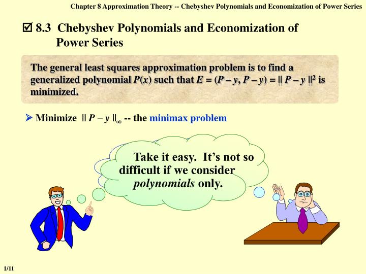
Chapter 8 Approximation Theory -- Chebyshev Polynomials and Economization of Power Series 8.3 Chebyshev Polynomials and Economization of Power Series The general least squares approximation problem is to find a generalized polynomial P(x) such that E = (P – y, P – y) = || P – y ||2 is minimized. Minimize || P – y || -- the minimax problem Take it easy. It’s not so difficult if we consider polynomials only. Didn’t you say it’s a very difficult problem? 1/11
Chapter 8 Approximation Theory -- Chebyshev Polynomials and Economization of Power Series Find a polynomialPn(x) of degreensuch that || Pn f|| is minimized. v 1.0 It is not easy to construct the polynomial from nowhere. However, we can examine the features of the polynomial: Definition: If P(x0) – f (x0) = || P f || , x0 is called a ()deviation point. If f C[a, b]and f is not a polynomial of degree n, then there exists a unique polynomialPn(x) such that || Pn f || is minimized. Pn(x) exists, and must have both + and – deviation points. Pn(x) f(x) has at least roots. (Chebyshev Theorem) Pn(x) minimizes || Pn f || Pn(x) has at least n+2 alternating + and – deviation points with respect to f. That is, there exists a set of points a t1 <…< tn+2 b such that Pn(tk) – f (tk) = (–1)k|| Pn f || . The set { tk } is called theChebyshev alternating sequence. n+1 2/11
Chapter 8 Approximation Theory -- Chebyshev Polynomials and Economization of Power Series v 2.0 y = + y f ( x ) E n = y P ( x ) n = y f ( x ) = - y f ( x ) E n Determine the interpolating points { x0, …, xn} such that Pn(x) minimizes the remainder x 0 Pn(x) is an interpolating polynomial of f(x) 3/11
Chapter 8 Approximation Theory -- Chebyshev Polynomials and Economization of Power Series Find { x1, …, xn } such that ||wn|| is minimized on [ 1, 1], where v 2.1 v 3.0 Find a polynomialPn–1(x) such that || xn – Pn–1(x)|| is minimized on [ 1, 1]. n = - w ( x ) ( x x ) n i = 1 i Notice that wn(x) = xn – Pn–1(x). The problem becomes to … From Chebyshev theorem we know that Pn1(x) has n+1 deviation points with respect to xn , that is, wn(x) obtains its maximum and minimum values alternatively on n+1 points. 4/11
Chapter 8 Approximation Theory -- Chebyshev Polynomials and Economization of Power Series cos(n ) assumes its maximum value 1 and minimum value 1 alternatively at points . And there exist coefficients a0, …, an such that Tn(x) assumes its maximum value 1 and minimum value 1 alter-natively at . That is, 1 Tn(x) has n roots Chebyshev polynomials Consider the extreme values of cos(n )on [ 0, ]. n + 1 Let x = cos( ), then x [ 1 , 1]. Tn(x) = cos( n) = cos( n · arc cos x ) is called the Chebyshev polynomial. More aboutTn: 5/11
Chapter 8 Approximation Theory -- Chebyshev Polynomials and Economization of Power Series v 3.0 Tn(x) is a polynomial of degree n with leading coefficient . { T0(x), T1(x), … } are orthogonal on [ 1 , 1] with respect to the weight function Find a polynomialPn–1(x) such that || xn – Pn–1(x)|| is minimized on [ 1, 1]. That is, Tn(x) has the recurrence relation: T0(x) = 1, T1(x) = x, Tn+1(x) = 2xTn(x) – Tn–1(x). 2n1 OKOK, I think it’s enough for us… What’s our target again? wn(x) = xn – Pn–1(x) = Tn(x) / 2n1 6/11
Chapter 8 Approximation Theory -- Chebyshev Polynomials and Economization of Power Series Find { x1, …, xn } such that ||wn|| is minimized on [ 1, 1], where v 2.1 v 2.0 n = - w ( x ) ( x x ) = { monic polynomials of degree n } n i = 1 i Determine the interpolating points { x0, …, xn} such that Pn(x) minimizes the remainder Take the n+1 roots of Tn+1(x) as the interpolating points { x0, …, xn }. Then the interpolating polynomial Pn(x) of f(x) assumes the minimum upper bound of the absolute error { x1, …, xn } are the n roots of Tn(x). 7/11
Chapter 8 Approximation Theory -- Chebyshev Polynomials and Economization of Power Series n = Example: Find the best approximating polynomial of f (x) = ex on [0, 1] such that the absolute error is no larger than 0.5104. Solution: Determine n: Make a change of the variable 4 Find the roots of T5(t): Make a change of the variable: Compute L4(x) with interpolating pointsx0, …, x4. 8/11
Chapter 8 Approximation Theory -- Chebyshev Polynomials and Economization of Power Series Given Pn(x) f (x), economization of power series is to reduce the degree of polynomial with a minimal loss of accuracy. Consider approximating an arbitrary n-th degree polynomial Pn(x) = anxn + an–1 xn–1 + … + a1x + a0 with a polynomial Pn–1(x) by removing an n-th degree polynomial Qn(x) that has the coefficient an for xn. Then - - + max | f ( x ) P ( x ) | max | f ( x ) P ( x ) | max | Q ( x ) | - 1 n n n - - - [ 1 , 1 ] [ 1 , 1 ] [ 1 , 1 ] Economization of Power Series To minimize the loss of accuracy, Qn(x) must be The loss of accuracy. 9/11
Chapter 8 Approximation Theory -- Chebyshev Polynomials and Economization of Power Series If we simply take , then the error is Example: The 4-th order Taylor polynomial for f (x) = ex on [1, 1] is The upper bound of truncation error is Please reduce the degree of the approximating polynomial to 2. Solution: 10/11
Chapter 8 Approximation Theory -- Chebyshev Polynomials and Economization of Power Series Note: A change of variable is needed for a general interval [a, b]. That is, let x = [(b – a)t + (a + b)]/2, then find the polynomial Pn(t) for f (t) on [1, 1] and finally obtain Pn(x). Another method is to write each term of xk as a linear combination of T0(x), …, Tk(x). For example, x = T1(x) and x3 = [T3(x) + 3 T1(x)] / 4. Then simply remove the Chebyshev functions from the original polynomial. HW: p.517 #3, 7, 9 11/11