Download
1 / 30
300 likes | 1.05k Views
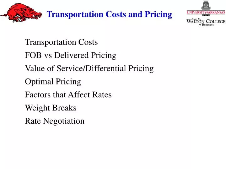
Transportation Costs FOB vs Delivered Pricing Value of Service/Differential Pricing Optimal Pricing Factors that Affect Rates Weight Breaks Rate Negotiation. Transportation Costs. Types of Costs Fixed Costs Variable Costs Common Costs Joint Costs Sources of Costs The Way

E N D
Transportation Costs FOB vs Delivered Pricing Value of Service/Differential Pricing Optimal Pricing Factors that Affect Rates Weight Breaks Rate Negotiation
Transportation Costs Types of Costs Fixed Costs Variable Costs Common Costs Joint Costs Sources of Costs The Way Terminals Vehicles
FOB vs Delivered Pricing Free on Board FOB Origin (Buyer Owns Goods in Transit) FOB Destination (Seller Owns Goods in Transit) Prepaid vs Collect/Allowed vs Charged Back Delivered Pricing Seller Retains Ownership in Transit Seller Arranges Transportation Seller Files Freight Claims Average Transportation Market Expansion Phantom Freight Freight Absorption
. C2 C1 FOB vs Delivered Pricing Delivered Price to all = $13/cwt FOB Plant= $10/cwt C1 pays more than fob Rate to C1= $2/cwt C2 is subsidized Rate to C2 = $4/cwt
Forms of FOB Pricing FOB Destination, Freight Allowed: Buyer is allowed to deduct the freight charges from the invoice. FOB Origin, Charged Back: Seller is allowed to add freight charges to the invoice. FOB Destination, Collect and Allowed: Buyer pays freight but deducts it from the invoice. FOB Origin, Prepaid and Charged Back: Seller pays the fright but adds it to the invoice.
Value of Service/Differential Pricing What is it? Why Use it? High Fixed Costs Excess Capacity Opportunity Competition When is it Profitable? When Above Full Cost When Below Full Cost If: Above Variable Cost Excess Capacity Elastic Demand
Unwise Truck Lines The Unwise Truck Lines Company operates five pieces of equipment daily over five routes with end points in common. The company just hired a new comptroller who is studying the profitability in order to determine which, if any, of the routes are not covering full costs, and, thus, not contributing to profits. He found that each route incurred $500 per day in variable operating expenses and earned the following revenue per day: Route 1 = $1,440; Route 2 = 1,220; Route 3 = 960; Route 4 = 800; Route 5 = 640. The new comptroller has stated that any route showing a loss after variable costs and a prorated share of overhead will be eliminated. Presently, the daily overhead is $1,500, or $300 per route. If any run is eliminated, overhead will decline by $50. Equipment will be sold to payoff any outstanding debt.
Should any routes be eliminated? Revenue Variable Over- Route per Run Cost/Run Gross head Net 1 1,440 (500) 940 (300) 640.00 2 1,120 (500) 620 (300) 320.00 3 960 (500) 460 (300) 160.00 4 800 (500) 300 (300) 0.00 5 640 (500) 140 (300) (160.00)
Eliminate Route 5 Revenue Variable Over- Route per Run Cost/Run Gross head Net 1 1,440 (500) 940 (362.50) 577.50 2 1,120 (500) 620 (362.50) 257.50 3 960 (500) 460 (362.50) 97.50 4 800 (500) 300 (362.50) (62.50)
Eliminate Route 4 Revenue Variable Over- Route per Run Cost/Run Gross head Net 1 1,440 (500) 940 (466.67) 473.33 2 1,120 (500) 620 (466.67) 153.33 3 960 (500) 460 (466.67) (6.67)
Eliminate Route 3 Revenue Variable Over- Route per Run Cost/Run Gross head Net 1 1,440 (500) 940 (675.00) 265.00 2 1,120 (500) 620 (675.00) (55.00) Eliminate Route 2 Revenue Variable Over- Route per Run Cost/Run Gross head Net 1 1,440 (500) 940 (1,300) (360.00) Eliminate Route 1
= 1 = Unitary Elasticity % % % Q Q Q E = E = E = % % % P P P > 1 = Elastic < 1 = Inelastic Price Elasticity of Demand Elasticity = Response in Quantity Sold to a Change in Price
P Elastic Unitary Inelastic Q Price Elasticity of Demand
Price Elasticity of Demand Changing Prices Increase price in an elastic market and decrease revenue Decrease in price in an elastic market and increase revenue Increase in price in an inelastic market and increase revenue Decrease in price in an inelastic market and decrease revenue
Optimal Pricing Maximize Profit Where: Marginal Cost Equals Marginal Revenue Which Financial Statement has Marginal Cost? Which Financial Statement has Marginal Revenue?
8 Zero Price, Large Q, 0* = 0 High Price, Zero Q, P*0 = 0 * Optimal Pricing Optimal Pricing Maximizing Revenue $ Inelastic Range Elastic Range Revenue Curve Price
Optimal Pricing Profit = Revenue - Cost (p = R - C) Revenue = Price * Quantity (R = P * Q) Cost = Fixed Cost + Variable Cost * Q (C = F + VQ) Quantity = a + bP (Q = a + bP) (p = R - C) (R = P * Q) (C = F + VQ) (Q = a + bP)
Optimal Pricing General Form of a Straight Line Y Y = a + bX b (Slope) Intercept a X
Optimal Pricing General Form of a Straight Line (Quantity Sold is Dependent upon Price) Q Q = a + bP b (Slope) Intercept a P
Optimal Pricing General Form of a Straight Line (Quantity Sold is Dependent upon Price) Q = a + bP However, the slope (b) is probably negative, but that must be determined)
Optimal Pricing p = [PQ - (F + VQ)] Q = a + bP p = [P(a + bP) - (F + V(a + bP))] p = [aP + bP2 - (F + aV + bVP)] p = aP + bP2 - F - aV - bVP To maximize Profit, set 1st derivative = zero, solve for P
-a V P* = + 2b 2 Optimal Pricing p = aP + bP2 - F - aV - bVP First Derivative = p' = [aP + bP2 - F - aV - bVP] To maximize Profit, set 1st derivative = zero, solve for P p' = a + 2bP - bV = 0 2bP = -a + bV
Slope = Zero Slope Negative * Optimal Pricing Profit = aP + bP2 - F - aV - bVP $ Profit Curve Slope Positive Price
Factors that Affect Rates Cost Related Commodity Factors Route Factors Demand Related Commodity Factors Route Factors
Factors that Affect Rates Cost Related Commodity Factors Loading Characteristics Susceptibility to Loss and Damage Volume of Traffic Regularity of Movement Equipment Requirements Route Factors Distance Operating Conditions Traffic Density Backhaul
Factors that Affect Rates Demand Related Commodity Factors Value of Commodity Economic Conditions of User Industry Competing Rates Route Factors Competition with Other Carriers Competition in Shipper Industry Competition in Receiver Industry Traffic Density
LTL $ TL Volume Weight Breaks A point of indifference between a given rate and a rate charged for a larger volume
Weight Breaks TL * MW = LTL * X Example: TL = $8.00/cwt MW = 40,000 LTL = $20.00 8*400 = 20* X 3200/20 = X X = 160 or 16,000 lbs If shipment is less than 16,000 lbs, ship LTL If shipment is over 16,000 lbs, ship TL as full TL (40,000lbs)
Rate Negotiation New Business Threat of Loss of Old Business Rule of Analogy (Protests) Bases of Power Reward Coercive Legitimate Referent Expert Know the Cost of Your Next Best Alternative
Determining Prices LTL vs TL Tapering Rates Class Rates Tariff Example