Download
1 / 57
570 likes | 649 Views
Upper bounds on k -SAT. Chris Calabro ccalabro@cs.ucsd.edu. What is k -SAT?. Variables – x 1 , x 2 , x 3 , … Literals – x 1 , ¬x 1 , x 2 , ¬x 2 ,… Clauses – (x 1 or ¬x 2 or x 3 ), (x 2 ), () CNFs – (x 1 or ¬x 2 or x 3 ) and (x 2 ) k-CNFs – (x 1 or ¬x 2 or x 3 ) and (x 2 ).

E N D
Upper bounds onk-SAT Chris Calabro ccalabro@cs.ucsd.edu
What is k-SAT? • Variables – x1, x2, x3, … • Literals – x1, ¬x1, x2, ¬x2,… • Clauses – (x1 or ¬x2 or x3), (x2), () • CNFs – (x1 or ¬x2 or x3) and (x2) • k-CNFs – (x1 or ¬x2 or x3) and (x2)
Assignment • (x1 or ¬x2 or x3) and (x2)
Assignment • (x1 or ¬x2 or x3) and (x2)
Assignment • (x1 or ¬x2 or x3) and (x2)
Formal problem • Decision version – k-SAT={F ε k-CNF | exists assignment a with F(a)=1} • Search version – given F ε k-CNF • find an assignment a with F(a)=1 • or output “not satisfiable” k-SAT ε NPC
Outline • Motivation • Why care about NPC problems? • Why upper bounds? • Why SAT? • How hard is SAT? • Algorithms • Design • Conclusion
NPC • Language L ε NPC iff • L ε NP • forall A ε NP, A ≤p L VERIFY={<M,x> | M is a Turing machine, x εΣ*, exists w εΣ|x|, M(x,w) accepts in time |x|} ε NPC • Solve L ε NPC efficiently => forall A ε NP, solve A efficiently • forall L ε NPC, (L ε P iff P=NP)
The big question • P = NP? • Posed by Kurt Gödel to John von Neumann in 1956 • Almost the same question: NP ≤ BPP?
Who cares? • Complexity theorists • Cryptographers • Engineers • Everybody else!
Possible worlds • P=NP? Unresolved • Theoreticians need to keep saying, “unless P=NP” • Could be wasting time on pointless theory • Can’t fully trust current crypto systems • P=NP • Poly hierarchy collapses: for each fixed m, can answer questions of form in poly time
If SAT ε DTIME(nk), k large • Crypto theory changes • No OWFs • No trapdoor functions • Crypto practice? Could there be a more efficient algorithm out there? • PRIMES ε DTIME(n12) [AKS02] • PRIMES ε RTIME(n3) [M76,R80] • What about BQP?
If SAT ε DTIME(nk), k small • No RSA, Diffie-Hellman, DES, AES, SHA1 • Symmetric key crypto not necessarily doomed • Info theoretically secure key exchange in bounded-storage model [AR99] • Quantum key exchange [BB84]
The good stuff • Test circuits/programs for correctness • Automatically generate proofs of mathematical theorems • Build better machines • Faster CPU • Perfect airplane wing • Solve AI problems
Black-box mistake-bounded learning • Online problem: at time t • Input – (x1,y1),…,(xt,yt) where |xi|=n, |yi|=1 coming from circuit C • Output – circuit Ct • Goal – Ct equivalent to C • Can bound # times t with Ct(xt+1)≠yt+1 by O(|C|2 lg|C|) • If |C| can be estimated, O(|C| lg|C|)
Why upper bounds? • Most researchers (61 to 9) think P≠NP [Gas02] • Why look for good upper bounds? There aren’t any, right? • NP problems could be easy in average case • There could be practical algorithms
Why SAT? • Why not subset sum, vertex cover, hampath, TSP? • Formulas look like natural language questions • Common problems efficiently reduce to SAT, often preserving structure of solution space • Many practical algorithms for SAT
An application • Circuit equivalence checking • Standard techniques – random simulation, BDDs • Alternative – reduce to SAT • [BCCFZ99] compared performance on real circuits with 1000s of gates
How hard is SAT? • Define • sk=inf{ε>0 | exists random alg A solving k-SAT in time O(2εn)} • σk=inf{ε>0 | exists random alg A solving unique k-SAT in time O(2εn)} • s∞=limk→∞ sk • σ∞=limk→∞σk • Exponential time hypothesis (ETH) – s3>0 forall k≥3 (ETH↔sk>0)
Outline • Motivation • Why care about NPC problems? • Why upper bounds? • Why SAT? • How hard is SAT? • Algorithms • Design • Conclusion
Outline • Motivation • Algorithms • Problem variants • Incremental assignment • Local search • Heuristics • Design • Conclusion
Problem variants • General k-SAT – worst case • Unique k-SAT – promise problem • YES – exactly 1 solution • NO – 0 solutions • Random k-SAT • Choose m random k-clauses with replacement • Plant a solution – choose random assignment a, then choose m clauses that agree with a • k-SAT from “real world” problem • Bounded model checking • Circuit fault analysis • Planning
Algorithmic paradigms • Incremental assignment (DPLL) – assign variables 1 at a time, simplifying formula as you go • Local search – choose an initial assignment, perform random walk directed by formula • Heuristics – combine features of other algorithms ad hoc
Incremental assignment Ordered-DLL(F) do t times for i=1,…,n choose unassigned var x at random if clause {x} ε F, assign x ← 1 else if {¬x} ε F, assign x ← 0 else assign x at random simplify F by removing true clauses, false literals if F=1, return assignment
Incremental assignment - analysis • Idea – lower bound probability p that each variable gets forced • Definition • Clause C ε F is critical at solution a iff C has exactly 1 true literal at a • Solution a is isolated iff flipping any variable in a yields a nonsolution • Claim – a isolated => F has ≥ 1 critical clause for each variable => p ≥ 1/k, conditioned on making random assignments in agreement with a
Incremental assignment - analysis • Corollary – a isolated => Pr(find a in 1 iteration) ≥ 2-(1-1/k)n • Either there is a nearly isolated solution or there are many solutions => running time ≤ poly(n)2(1-1/k)n [PPZ97] • Strengthened analysis – poly(n)(2n/s)1-1/k [CIKP03]
Resolution • Each clause provides info about solution set • Why not add preprocessing step that adds clauses implied by formula F? • (x1 or α) and (¬x1 or β) => α or β • Definition – F is fully resolved iff F is closed under resolution
Resolution is complete • Let S = solution space of formula F • Definition – variable x is determined iff • forall a ε S, a(x)=1 • or forall a ε S, a(x)=0 • Theorem – let F be fully resolved, x be a variable, b ε {0,1}, then • F is satisfiable iff ¬(Ø ε F) • x is determined iff F contains a unit clause in x • F|x←b is fully resolved
Bounded resolution • Problems with full resolution • Resolvent of 2 k-clauses could have size 2k-2 • Exponentially many large clauses • Shortest resolution refutation of unsatisfiable formulas may be exponentially large • Simple solution – s-bounded resolution • For some constant s, produce resolvent R only if |R| ≤ s
Resolve SAT • Algorithm – preprocess F by performing s-bounded resolution (s=O(lg n)), then use ordered-DLL • Bound improves from poly(n)2(1-1/k)n to poly(n)2(1-μk/(k-1))n where , k≥5 • Same bound for unique k-SAT, k≥3 • Best k-SAT alg for k≥4. O(2.5625n) for k=4. • Best unique k-SAT alg for k≥3. O(2.3863n) for k=3.
Local search Local-search(F) do t times choose random assignment a do 3n times if F(a)=1, return a choose an unsatisfied clause C choose var x in C at random flip x in a
Local search - analysis • Let z be a particular solution • Can model each iteration as a Markov process • States – 0,1,2,… • State i represents dist(a,z)=i • State 0 is absorbing • Initial state is binomial (n,1/2), then algorithm performs a random walk
Local search - analysis • Let z be a particular solution • Can model each iteration as a Markov process • States – 0,1,2,… • State i represents d(a,z)=I • State 0 is absorbing • Initial state is binomial (n,1/2), then algorithm performs a random walk 0---1---2---3---4---5---6---7---…
Local search - analysis • Let z be a particular solution • Can model each iteration as a Markov process • States – 0,1,2,… • State i represents d(a,z)=I • State 0 is absorbing • Initial state is binomial (n,1/2), then algorithm performs a random walk 0---1---2---3---4---5---6---7---…
Local search - analysis • Let z be a particular solution • Can model each iteration as a Markov process • States – 0,1,2,… • State i represents d(a,z)=I • State 0 is absorbing • Initial state is binomial (n,1/2), then algorithm performs a random walk 0---1---2---3---4---5---6---7---…
Local search - analysis • Let z be a particular solution • Can model each iteration as a Markov process • States – 0,1,2,… • State i represents d(a,z)=I • State 0 is absorbing • Initial state is binomial (n,1/2), then algorithm performs a random walk 0---1---2---3---4---5---6---7---…
Local search - analysis • Let z be a particular solution • Can model each iteration as a Markov process • States – 0,1,2,… • State i represents d(a,z)=I • State 0 is absorbing • Initial state is binomial (n,1/2), then algorithm performs a random walk 0---1---2---3---4---5---6---7---…
Local search - analysis • Let z be a particular solution • Can model each iteration as a Markov process • States – 0,1,2,… • State i represents d(a,z)=I • State 0 is absorbing • Initial state is binomial (n,1/2), then algorithm performs a random walk 0---1---2---3---4---5---6---7---…
Local search - analysis • Let z be a particular solution • Can model each iteration as a Markov process • States – 0,1,2,… • State i represents d(a,z)=I • State 0 is absorbing • Initial state is binomial (n,1/2), then algorithm performs a random walk 0---1---2---3---4---5---6---7---…
Local search - analysis • Let z be a particular solution • Can model each iteration as a Markov process • States – 0,1,2,… • State i represents d(a,z)=I • State 0 is absorbing • Initial state is binomial (n,1/2), then algorithm performs a random walk 0---1---2---3---4---5---6---7---…
Local search - analysis • Pr(go left) ≥ 1/k • Pr(go right) ≤ 1-1/k • Let p = Pr(reach 0 in one iteration) • Naïve analysis – p ≥ Pr(reach 0 by successive left moves) ≥ • Better analysis – use reflection principle to show p ≥ • Running time – [Sch99]
Heuristics • Complete – gives correct answer with probability 1 (satz, SATO, zChaff) • Incomplete – sometimes fails to find witness • Probabilistically Approximately Complete (PAC) – succeed with probability 1 without restarts if given enough time (UnitWalk) • Essentially incomplete – succeed with probability <1 unless restarted (GSAT, GWSAT, HSAT, HWSAT, WalkSAT)
UnitWalk choose initial assignment a do t times use ordered-DLL (with a as randomness!) to find next assignment
Variants • UnitWalk+WalkSAT – alternate steps of UnitWalk and WalkSAT! • UnitWalk+incBinSAT+WalkSAT – add preprocessing step of 2-bounded resolution • Common benchmarks • Random formulas, circuit problems, bounded-model checking, planning problems • Variables and clauses – 100s to 10,000s • Running times – seconds to minutes
Outline • Motivation • Algorithms • Problem variants • Incremental assignment • Local search • Heuristics • Design • Conclusion
Outline • Motivation • Algorithms • Design • Sparsification • Isolation • Conclusion
Sparsification • Given k-CNF F, ε > 0, we can generate in time poly(n)2εn a disjunction G of 2εn k-CNFs Gi, each of size O(n) [IPZ98] • Each Gi can be produced in time poly(n) • Can be used as a preprocessing step when • Algorithm is exponential time anyway • Linear sized formulas are needed
Sparsification example • Theorem – σ3 = 0 => s∞ = 0 [CIKP03] • Proof shows a reduction from general k-SAT to unique 3-SAT • To do this requires clause width reduction • Standard algorithm produces formula with O(n+m) variables (m = #clauses in input formula) • Sparsify first! Then O(n+m)=O(n)