Download
1 / 31
320 likes | 563 Views
How to use Matlab. 27- 750 Texture, Microstructure & Anisotropy A.D. Rollett. Last revised: 25 th Feb. ‘14. In-Class Questions. What is the procedure that one can follow to use Matlab+MTex to construct an orientation distribution from pole figure data?

E N D
How to use Matlab 27-750 Texture, Microstructure & Anisotropy A.D. Rollett Last revised:25thFeb. ‘14
In-Class Questions • What is the procedure that one can follow to use Matlab+MTex to construct an orientation distribution from pole figure data? • What is the procedure that one can follow to use Matlab+MTexto construct an orientation distribution from EBSD data? • What else can one obtain from a Matlab+MTex analysis?
Installation of MTex • Find MTEX by searching on “mtexgoogle code” • MTex has its own installation procedure. As detailed in the instructions found on-line, the steps include a) set the Matlab “path” to the folder/directory where the MTex package is located; b) in the Matlab command window, type “startup_mtex”. • Fortunately, this takes care of replacing any previous, older installations of MTex. • The Matlab documentation will now include documentation on MTex. • Caution: if you manually add the MTEX folder to your MATLAB path then there is a significant risk that MTEX will give errors (e.g. when you try to read in EBSD data). What you should do instead to get it to work is to put MTEX in a different folder and run startup_mtex from that directory. DO NOT add it to the search path!
What can MTex do? • We will explore two things: a) analysis of pole figure data; b) analysis of EBSD data. • Useful links:This one describes ways to plot individual orientations.http://merkel.zoneo.net/RDX/index.php?n=Texture.PlotIndividualOrientationsInMTex
Navigating the file structure >> pwdwill tell you which directory you are in (probably “~/Documents/MATLAB”>> cd /directory-of-your-choicewill place you in whatever folder/directory you like, i.e. where you have your data.You can then click on “Import pole figure data” or “Import EBSD data”, for example, to set up the script to read in your data.
PF analysis • Look in the “Mtex Toolbox” for “Short Pole Figure Analysis Tutorial”. Do not use this! • Instead, type import_wizard • A new, small window will open. It should be set to the “Pole Figures” tab by default (but if not, click on that tab).Click on the “+” and navigate to where you have “alr.epf” stored.You should see the window below.
PF analysis – p2 • Click on “Next >>” in the same window. You can enter the lattice parameter as 4.05 if you wish (although it should not make any difference because this is cubic).The wizard is quite clever: if you enter “Fe” as the mineral name, it will recognize this material and make the appropriate entries for you.
PF analysis – p3 • I prefer to set the plotting axes so that “x” points to the right (East), as for normal plots. For now re-set the “specimen symmetry” to “orthorhombic”.
PF analysis – p4 • After clicking “Next >>”, you should see this window.
PF analysis – p5 • After clicking “Next >>”, you should see this window (but with “orthorhombic” for the sample symmetry). Now click “Finish” to be done.
Plot experimental PFs • Plot(pf) should show you discrete pole figures; “pf” was the default name of the PF data that you read in.
ODF analysis • At this point you can run the ODF analysis: odf = calcODF(pf) ------ MTEX -- PDF to ODF inversion ------------------ Call c-routine initialize solver start iteration error: 7.1530E-01 4.2632E-01 2.1810E-01 1.3615E-01 9.8065E-02 7.7246E-02 7.1090E-02 6.7171E-02 6.4644E-02 6.2644E-02 6.0870E-02 Finished PDF-ODF inversion. error: 6.0870E-02 alpha: 1.0518E+00 1.0678E+00 1.1113E+00 required time: 6s odf = ODF (show methods, plot) comment: ODF recalculated from /Users/rollett/Word/teaching/Micro14/MatLab_Casper/Al-PFs/alr.epf crystal symmetry: aluminum (m-3m) sample symmetry : orthorhombic Radially symmetric portion: kernel: de la ValleePoussin, hw = 5° center: 1232 orientations, resolution: 5° weight: 1
Recalculated PFs • Type “plotpdf(odf,h,'antipodal')” to plot the same set of pole figures but based on the ODF. Note that these are quadrant PFs because of the assumed orthorhombic sample symmetry.
Adjust sample symmetry • Now go into the script that you had generated for the PF import, and change (by editing it) the sample symmetry from orthorhombic to triclinic.
Re-analyze • Re-run the calcODF and plotpdf commands.
Inverse PFs • To get a complete set of 3 inverse pole figures, type “plotipdf(odf,[xvector,yvector,zvector],'antipodal')”. The 3 sample directions are specified by the built-in “xvector”, “yvector” and “zvector”.
Sections through ODF • plot(odf,’PHI2’,'sections') will give you plots of sections through the ODF. These go to 360° in phi1, because of the triclinic sample symmetry.
3D view • “plot(odf,'PHI2','surf3')” – gives rotatable view.
Misc. >> textureindex(odf) ans = 10.6263>> entropy(odf) ans = -1.6371 • These values suggest a moderately strong texture. • The section on “Characterizing ODFs” provides a few other techniques.
Errors %Error analysis: %For a more quantitative description of the reconstruction quality one can use the function calcError to compute the fit between the reconstructed ODF and the measured pole figure intensities. The following measured are available: RP - error ; L1 – error; L2 – error calcError(pf,odf,'RP',1) ans= 0.1540 0.1631 0.1319 0.1033 0.1163 0.1763 0.1734 %In order to recognize bad pole figure intensities it is often useful to plot difference pole figures between the normalized measured intensities and the recalculated ODF. This can be done with the command PlotDiff. plotDiff(pf,odf)
Volume fraction First we specify an texture component using “orientation”: ori = orientation('Euler',phi1,Phi,phi2,cs,ss) e.g. center = orientation('Euler’,0,55,45,CS,SS) The function 'volume' returns the ratio of an orientation that is close to an orientation (center) by a misorientation tolerance (radius) to the volume of the entire odf. Syntax: v = volume(odf,center,radius,<options>)
EBSD input • Navigate with “cd” to wherever your data is; in this case, you need to download fw-ar-IF1-avtr12-corr.ctf from the CMU box for 27-750. You are recommended to place it in a folder/directory by itself so that you can store the images from running Matlab+MTEX. On the Macs, “Grab” is v handy for screen/window captures. • Click on “Import EBSD data”, just as you did for the pole figure data and follow the steps to specify the material etc. • This generates a dataset called “ebsd”. • Type “plot(ebsd,'colorcoding','ipdfHKL')” • This will give a map of the material that is colored by the crystal plane exposed at the surface.
EBSD: get grains • Type “grains = calcGrains(ebsd)” • Then re-plot the ipdfHKL map and add grain boundaries:plot(ebsd,'colorcoding','ipdfHKL’)hold onplotBoundary(grains,'linewidth',1.5) • This will provide a similar map but with the GBs delineated.
Average grain orientations • plot(grains,'colorcoding','ipdfHKL')
ODF from EBSD First, do this: plot(ebsd,'property','phase') psi = calcKernel(grains('Fe')) odf = calcODF(ebsd('Fe'),'kernel',psi)The first should be “boring” i.e. it should show only 1 phase. The second should show a few lines of output with details about the calculation. The third is the calculation of the ODF.
Plot pole figures h = [Miller(1,0,0),Miller(1,1,0),Miller(1,1,1)]; This defines a setof pole figureindices plotpdf(odf,h,'antipodal') This shows a setof PFs based on thecalculated ODF.
ODF plots plot(odf,'PHI2','surf3') This shows a 3D viewofthe ODF; 2 viewsshown
ODF sections in f2 These show a clear gamma fiber, albeit imperfect. This is characteristic of a rolled bcc metals.
Inv. PFs plotipdf(odf,[xvector,yvector,zvector],'antipodal') Note how the 001 inverse pole figure shows a strong maximum at the <111> position.
Additional Steps • Eliminate small grains:% correct for too small grains grains = grains(grainSize(grains)>5);
Summary • The sequence provided up to this point illustrates how to read in and perform standard analysis on pole figures.