Download
1 / 30
330 likes | 600 Views
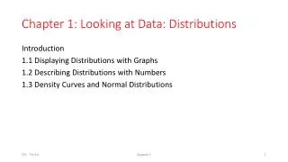
Looking at data: distributions - Density curves and normal distributions. IPS section 1.3. © 2006 W.H. Freeman and Company (authored by Brigitte Baldi, University of California-Irvine; adapted by Jim Brumbaugh-Smith, Manchester College). Objectives. Density Curves and Normal Distributions

E N D
Looking at data: distributions- Density curves and normal distributions IPS section 1.3 © 2006 W.H. Freeman and Company (authored by Brigitte Baldi, University of California-Irvine; adapted by Jim Brumbaugh-Smith, Manchester College)
Objectives Density Curves and Normal Distributions • Understand interpretation of density curves • Understand characteristics of normal distributions • Apply the 68-95-99.7 Rule • Compute and interpret a z-score for normal data • Calculate normal probabilities • Calculate normal percentiles • Compare values from different normal populations • Assess normality of data using normal quantile plots
Terminology • Density curve (or “probability density function”) • Normal distributions (or “normal curves” • The “68-95-99.7 Rule” (or the “Empirical Rule”) • Standard normal distribution • Standardized value (or “z-score”) • Normal quantile plot
Density curves A density curve is a mathematical model of a distribution. It can be thought of as a smoothed version of the underlying histogram. It is always on or above the horizontal axis. The total area under the curve, by definition, is equal to 1, or 100%. The area under the curve for a range of values is the proportion of all observations within that range. Histogram of sample data with theoretical density curve describingthe population
Density curves can come in any imaginable shape (as long as the area beneath equals 1). Some are well-known mathematically and others aren’t. As with histograms, peaks represent ranges with frequently occurring values while valleys and tails correspond to less frequently occurring values.
Normal distributions Normal (or “Gaussian”) distributions are a family of symmetric, single-peaked density curves defined by the mean m (mu) and standard deviation s (sigma). A normal distribution is symbolized by N (m, s). x x While not essential to know, the above equation represents the red normal curve. e = 2.71828… (the base of the natural logarithm) π = pi = 3.14159…
A family of normal curves Here the means are different (m = 10, 15, and 20) while the standard deviations are all the same (s = 3). Visually, how can you tell all three curves have the same standard deviation of s = 3 ? Which of the above corresponds to the normal curve with mean of m = 10 ?
A family of normal curves Here the means are the same (m = 15) while the standard deviations are different (s = 2, 4, and 6). Visually, how can you tell that all three curves have the same mean of m = 15 ? Which of the above corresponds to the normal curve with standard deviation of s = 6?
Characteristics of any normal curve • a normal curve defined by its mean m and std. deviation s • larger s implies more variation in the data, so the normal curve will be broader • exactly symmetric and single peaked • in theory, no lower or upper limit on data represented • curvature changes at m−s and m + s • total area beneath equals 1 • area on either side of mean is .50 (due to symmetry) • area beneath represents probability
The 68-95-99.7 Rule for normal distributions • About 68% of all observations are within 1 standard deviation of the mean. 64.5 ± 1(2.5) → 64.5 ± 2.5 → 62 to 67 inches • About 95% of all observations are within 2 s of the mean. 64.5 ± 2(2.5) → 64.5 ± 5 → 59.5 to 69.5 inches • Almost all (99.7%) observations are within 3 s of the mean. 64.5 ± 3(2.5) → 64.5 ± 7.5 → 57 to 72 inches Inflection point mean µ = 64.5 standard deviation s = 2.5 N(µ, s) = N(64.5, 2.5) Reminder: µ (mu) is the mean of the idealized normal curve, while is the mean of a sample. σ (sigma) is the standard deviation of the idealized curve, while s is the std deviation. of a sample.
N(64.5, 2.5) N(0,1) => Standardized height (no units) The standard normal distribution Because all normal distributions share the same properties, we can standardize our data to transform any normal curve N (m, s) into the standard normal curveN (0,1). For any x we can calculate a “standardized value” z (called a z-score).
Standardizing: calculating z-scores How tall is X=67 inches compared to the mean of 64.5? Clearly it is 2.5 inches above average. (X−m = 67−64.5 = 2.5) But how far is it above the mean relative to the standard deviation? A z-score measures the number of standard deviations that a data value x is from the mean m. • When X is larger than the mean, z is positive. • When X is smaller than the mean, z is negative. • For the mean itself, z=0.
Example: Women heights N(µ, s) = N(64.5, 2.5) Women’s heights follow the N(64.5″,2.5″) distribution. What percent of women are shorter than 67 inches tall (that’s 5′7″)? Area= .50 Area= ??? Area = ??? Area = .34 mean µ = 64.5" standard deviation s = 2.5" X (height) = 67" m = 64.5″ X = 67″ z = 0 z = 1 We calculate z, the standardized value of x: Using the 68-95-99.7 rule, we can conclude that the percent of women shorter than 67″ is approximately, .50 + (half of .68) = .50 + .34 = .84, or 84%.
Using Table A to find percent of women shorter than 67” The area under the standard normal curve to the left of z =1.00 is 0.8413. N(µ, s) = N(64.5”, 2.5”) Area ≈ 0.84 Conclusion: 84.13% of women are shorter than 67″. (By subtraction, 1 − 0.8413, or 15.87%, of women are taller than 67".) Area ≈ 0.16 m = 64.5” x = 67” z = 1
.0082 is the area under N(0,1) left of z = -2.40 0.0069 is the area under N(0,1) left of z = -2.46 .0080 is the area under N(0,1) left of z = -2.41 Using Table A Table A gives the area under the standard normal curve to the left of any z-score. (…)
area right of z = 1 − area left of z Using Table A to find right-hand areas Since the total area is 1, right-hand area = 1 − left-hand area
The National Collegiate Athletic Association (NCAA) requires Division I athletes to score at least 820 on the combined math and verbal SAT exam to compete in their first college year. The SAT scores of 2003 were approximately normal with mean 1026 and standard deviation 209. What proportion of all students would be NCAA qualifiers (SAT ≥ 820)? Area right of 820 = Total area − Area left of 820 = 1 − 0.1611 = .8389 ≈ 84% Note: The actual data may contain students who scored exactly 820 on the SAT. However, the proportion of scores exactly equal to 820 is considered to be zero for a normal distribution due to the idealized smoothing of density curves.
Using Table A to find in-between areas To calculate the area between two X values: a) compute their z-scores separately. b) find the area to the left of each z-score. c) subtract the smaller area from the larger area. area between z1 and z2 = (area left of z1) – (area left of z2) A common mistake is to subtract the z-scores; only subtract areas.
The NCAA defines a “partial qualifier” (eligible to practice and receive an athletic scholarship but not to compete) as a combined SAT score of at least 720. What proportion of all students who take the SAT would be partial qualifiers? That is, what proportion have scores between 720 and 820? Area in between = Area left of 820 − Area left of 720 = 0.1611 − 0.0721 = .8900 ≈ 9% About 9% of all students who take the SAT have scores between 720 and 820.
Comparing Apples to Oranges When working with normally distributed data we can manipulate it and then compare seemingly non-comparable distributions. We do this by “standardizing” the data. This involves changing the scale so that the mean now equals 0 and the standard deviation equals 1. If you do this to different distributions, it makes them comparable. N(0,1)
Who is “taller”? A 67-inch woman or a 71-inch man? Women’s Heights ~ N(64.5”, 2.5”) Men’s Heights ~ N(69”, 2.5”) We already saw a 67” women is 1 std. deviation above the mean for women. How many std. deviations above the mean is 71” man? (compared to the male mean)
What improvement did we get by adding better food? Example: Gestation time in malnourished mothers What are the effects of better maternal care on gestation time and premies? The goal is to obtain pregnancies of 240 days (8 months) or longer. • 266 s 15 • 250 s 20
Under each treatment, what percent of mothers failed to carry their babies at least 240 days? Vitamins only m = 250, s = 20, x = 240 Vitamins only: 30.85% of women would be expected to have gestation times shorter than 240 days.
Vitamins and better food m= 266, s= 15, x = 240 Vitamins and better food: 4.18% of women would be expected to have gestation times shorter than 240 days. Compared to vitamin supplements alone, vitamins and better food resulted in a much smaller percentage of women with pregnancy terms below 8 months (4% vs. 31%).
Determining normal percentiles Find the height (X) such that 25% of women are below this height. That is, find the 25th percentile for women’s heights. When you know the desired percentage, but you don’t know the X value that represents the cut-off, you need to use Table A backward. • Find the percentile (left-hand area) in the body of Table A. • Find the corresponding z-score in the margin of Table A. • 3. Transform Z back to the X scale (that is, inches). Plug in m, s and Z and then solve for X.
Example: Women’s heights Women’s heights follow the N(64.5″,2.5″) distribution. What is the 25th percentile for women’s heights? mean µ = 64.5" standard deviation s = 2.5" proportion = area under curve = 0.25 On the first page of Table A, a left-hand area of 0.25 corresponds to z = −0.67 (closest area is .2514). −.67(2.5) = X − 64.5 or X = 64.5 −.67(2.5) = 62.825 The 25th percentile for women’s heights is roughly 62.8”.
Assessing normality • In problem solving we often assume data is normal. • In statistical work we often need to verify that data is close to normal. • Is the data in the following histogram fairly normal? • The overall shape is fairly symmetric with one main peak in the center. • Recall that histograms can be misleading depending on the number of vertical bars used. • Adding the best fitting normal curve N(100, 9.7) suggests a fairly good fit.
Normal quantile plots A normal quantile plot (Q-Q plot in SPSS) is a plot of z-scores versus the actual data (X). If the data is close to normal than the quantile plot will be close to linear. • Here the plot very closely follows the diagonal reference line indicating the data is close to normal. • We generally ignore any slight irregularities at the ends. • Points off to the far left or right indicate outliers.
More quantile plots – skewed data Quantile plots for skewed data show a sweeping curve. Concave down → skewed right Concave up → skewed left These descriptions apply to SPSS. In figures from our textbook (IPS) the direction of the skewness is the opposite.
More quantile plots – symmetric, non-normal data Quantile plots for symmetric, but non-normal data show an S shape. Backwards S → symmetric but with shorter tails than normal Regular S → symmetric but with longer tails than normal These descriptions apply to SPSS. In figures from our textbook (IPS) the length of the tails is the opposite.