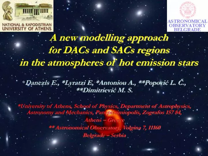
A new modelling approach for DACs and SACs regions in the atmospheres of hot emission stars

1. A new modelling approachfor DACs and SACs regionsin the atmospheres of hot emission stars *Danezis E., *Lyratzi E, *Antoniou A., **Popović L. Č., **Dimitriević M. S. *University of Athens, School of Physics, Department of Astrophysics, Astronomy and Mechanics, Panepistimiopolis, Zografos 157 84, Athens – Greece ** Astronomical Observatory, Volgina 7, 11160 Belgrade – Serbia

2. The GR model One of the main hypotheses when we constructed an old version of our model (rotation model), was that the line’s width is only a rotational effect and we considered spherical symmetry for the independent density regions. In a new approach of the problem we also consider the random velocitiesin the calculation of the distribution function L that we can detect in the line function. This newLis a synthesis of the rotational distribution Lr that we had presented in the old rotational model and a Gaussian that well defines the random velocities. This means that the new L has two limits, the first one gives us a Gaussian and the other the old rotation distribution Lr.

3. V Ai (λlab) φ Vrad φ equator The new calculation of the distribution functions L Let us consider a spherical shell and a point Ai in its equator. If the laboratory wavelength of a spectral line that arises from Ai is λlab, the observed wavelength will beλ0=λlab+Δλrad Danezis, E., Lyratzi, E., Nikolaidis, D., Antoniou, A., Popović, L. Č. & Dimitrijević, M. S.,2007 PASJ, 59, 4

4. φ Vrot Ai (λ0) φ The calculation of the distribution functions L If the spherical density region rotates, we will observe a displacement Δλrot and the new wavelength of the center of the line λi is: where where is the observed rotational velocity of the point Ai. This means that and if then

5. If we consider that the spectral line profile is a Gaussian, then we have: where κis the mean value of the distribution and in the case of the line profile it indicates the center of the spectral line that arises from Ai. This means that:

6. For all the semi-equator we have If we make the transformation , and the above function (4) will be transformed and finally we have the function (5) :

8. The above integrals have the form of a known integral erf(x) that has the following properties: 1. 2. 3.as 4. 5. 6.

9. (6) The distribution function from the semi-spherical region is: (7) (Method Simpson) This Lfinal(λ) is the distribution that replaces the old rotational distribution L that our group proposed some years ago (Danezis et al 2001).

10. Discussion In the proposed distribution an important factor is This factor indicates the kind of the distribution that fits the line profile. 1. If we have a mixed distribution. The line broadening is an effect of two equal reasons: a. The rotational velocity of the spherical region and b. The random velocities of the ions.

11. If m ≈ 500 the line broadening is only an effect of the • rotational velocity and the random velocities are very low. • In this case the profile of the line is the same with • the profile that we can produce using the old rotation model • (Danezis 2001, 2003).

12. Finally, if m<1the line broadening is only an • effect of random velocities • and the line distribution is a Gaussian.

13. The column density An important point of our study is the calculationof thecolumn densityfrom our model. Lets start from the definition of the optical depth: where τ is the optical depth (no units), k is the absorption coefficient ( ), ρ is the density of the absorbing region ( ), sis the geometrical depth (cm) Danezis, E., Lyratzi, E., Nikolaidis, D., Antoniou, A., Popović, L. Č. & Dimitrijević, M. S.,2007 PASJ, 59, 4

14. In the model we set , so whereLis the distribution function of the absorption coefficient k and has no units, Ω equals 1 and has the units of k ( ) We consider that for the moment of the observation and for a significant ion, k is constant, so k (and thus L and Ω) may come out of the integral. So: We set and τ becomes

15. Absorption lines For every one of ξ along the spectral line (henceforth called ξi) we have that: We set As contributes only to the units, σitakes the value of ξi. For each of λialong the spectral line, we extract a σi from each ξi. The program we use calculates the ξi for the centre of the line. This means that from this ξiwe can measure the respective σi.

16. If we add the values of all σi along the spectral line then we have ( in ), which is the surface density of the absorbing matter, which creates the spectral line. If we divide σ with the atomic weight of the ion which creates the spectral line, we extract the number density of the absorbers, meaning the number of the absorbers per square centimetre ( (in )).

17. This number density corresponds to the energy density which is absorbed by the whole matter which creates the observed spectral line( (in )) and which is calculated by the model. It is well known, that each absorber absorbs the specific amount of the energy needed for the transition which creates the specific line. This means that if we divide the calculated energy density ( ) with the energy needed for the transition, we obtainthe column density (in ).

18. Emission lines In the case of the emission lines we have to take into account not only ξe, but also the source function S, as both of these parameters contribute to the height of the emission lines. So in this case we have: where: j is the emission coefficient ( ), kis the absorption coefficient ( ) ρe is the density of the emitting region ( ) s is the geometrical depth (cm)

19. We set where L is the distribution function of the absorption coefficient k and has no units, Ω equals 1 and has the units of k ( ) And where Leis the distribution function of the emission coefficient j and has no units, Ωeequals 1 and has the units of j As we did before, in the case of the absorption lines, we may consider that Ωmay come out of the integral.

20. So: As in the model we use the same distribution for the absorption and for the emission, . So: We set As contributes only to the units, σe takes the value of Sξe.

21. For each λi along the spectral line, we extract a σi from each Sξe. The program we use calculates the ξefor the center of the line and the S. This means that from this ξe and S we can measure the respective σi. If we add the values of all σi along the spectral line then we have (in ), which is the surface density of the emitting matter, which creates the spectral line. If we divide σwith the atomic weight of the ion which creates the spectral line, we extract the number density of the emitters, meaning the number of the emitters per square centimetre (in ).

22. This number density corresponds to the energy density which is emitted by the whole matter which creates the observed spectral line ( (in )) and which is calculated by the model. It is well known, that each emitter emits the specific amount of the energy needed for the transition which creates the specific line. This means that if we divide the calculated energy density( ) with the energy needed for the transition, we obtain the column density (in ).

23. The next presentation is about some important remarks and applications of GR model

24. Thank you very much for your attention