Download
1 / 58
690 likes | 1k Views
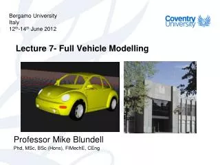
Bergamo University Italy 12 th -14 th June 2012. Lecture 7- Full Vehicle Modelling. Professor Mike Blundell Phd , MSc, BSc ( Hons ), FIMechE , CEng. Contents. Underlying Theory (Bicycle Model Approach) Understeer and Oversteer

E N D
Bergamo University Italy 12th-14th June 2012 Lecture 7- Full Vehicle Modelling Professor Mike Blundell Phd, MSc, BSc (Hons), FIMechE, CEng
Contents • Underlying Theory (Bicycle Model Approach) • Understeer and Oversteer • Modelling Strategies (Lumped Mass, Swing Arm, Roll Stiffness, Linkages) • Vehicle Body Measurements and Influences
Underlying Theory - Bicycle Model O1 Vy2 X1 • The simplest possible representation of a vehicle manoeuvering in the ground plane (bicycle model) • Weight transfer • Tyre lateral force characteristics as a function of tyre load GRF Vx2 Y1 Y2 X2 O2 G2 Fy wz2 Fy
Vehicle Handling “Handling” is • different to maximum steady state lateral acceleration (“grip”) • much less amenable to a succinct definition • “a quality of a vehicle that allows or even encourages the operator to make use of all the available grip” • (Prodrive working definition) • Emotional definitions like: “Confidence” (Consistency/Linearity to Inputs) “Fun” (High Yaw Gain, High Yaw Bandwidth) “Fluidity” (Yaw Damping Between Manoeuvres) “Precision” (Disturbance Rejection) Courtesy of www.drivingdevelopment.co.uk
w Vehicle Handling “Inertia Match” is the relationship between the CG position, wheelbase and yaw inertia. At the instant of turn in: w= Cafaf a t / Izz v = Cafaf t / m Combining these velocities gives an “instant centre” at a distance c behind the CG: c = Izz/ ma Noting that Izz = mk2 Thus if c is equal to b then 1 = k2 / ab u v a b c
Vehicle Handling k2/ ab therefore describes the distance of the centre of rotation with respect to the rear axle. • It is referred to as the “Dynamic Index” • DI fraction is length ratio c / b • DI > 1 implies c > b • DI < 1 implies c < b • Magic Number = 0.92 a b c
Roll Angle Lateral Acceleration (Ay ) Forward Speed (Vx) Vehicle Handling – Understeer and Oversteer For pure cornering (Lateral Response) the following outputs are typically studied: • Lateral Acceleration (g) • Yaw Rate (deg/s) • Roll Rate (deg) • Trajectory ( Y (mm) vs. X (mm)) Typical lateral responses measured in vehicle coordinate frame
L do Centre of Mass t di R Centre of Turn Cornering at Low-Speed Assuming small steer angles at the road wheels to avoid scrubbing the wheels The average of the inner and outer road wheel angles is Known as the Ackerman Angle
Steady State Cornering • Start with a simple ‘Bicycle’ model explanation • The model can be considered to have two degrees of freedom (yaw rotation and lateral displacement) No roll! • In order to progress from travelling in a straight line to travelling in a curved path, the following sequence of events is suggested: • The driver turns the hand wheel, applying a slip angle at the front wheels • After a delay associated with the front tyre relaxation lengths, side force is applied at the front of the vehicle • The body yaws (rotates in plan), applying a slip angle at the rear wheels
c b ar af d R Centre of Turn Steady State Cornering (continued) • After a delay associated with the rear tyre relaxation lengths, side force is applied at the rear of the vehicle • Lateral acceleration is increased, yaw acceleration is reduced to zero
Bicycle Model Simplified c b αr X αf δ Fry Ffy Y m ay The bicycle model can be described by the following two equations of motion: Ffy + Fry = m ay Ffy b - Fry c = 0
Understeer Path Neutral Steer Path Oversteer Path Disturbing force (e.g. side gust) Acting through the centre of mass Understeer and Oversteer Olley’s Definition (1945)
Neutral Steer Understeer Oversteer Understeer and Oversteer • Understeer promotes stability • Oversteer promotes instability (spin)
V ay 33 m The Constant Radius Test The constant radius turn test procedure can be use to define the handling characteristic of a vehicle (Reference the British Standard) • The procedure may be summarised as: • Start at slow speed, find Ackerman angle • Increment speed in steps to produce increments in lateral acceleration of typically 0.1g • Corner in steady state at each speed and measure steering inputs • Establish limit cornering and vehicle Understeer / Oversteer behaviour ay = V2 / R
δ (deg) Understeer Ackerman Angle K = Understeer Gradient Oversteer Lateral Acceleration (g) Understeer Gradient • It is possible to use results from the test to determine Understeer gradient • Use steering ratio to establish road wheel angle d from measured hand wheel angles • At low lateral acceleration the road wheel angle d can be found using: • Where: • δ = road wheel angle (deg) • K = understeer gradient (deg/g) • Ay = lateral acceleration (g) • L = track (m) • R = radius (m)
δ (deg) Limit Understeer Neutral Steer Limit Oversteer Vehicle 1 Vehicle 2 Lateral Acceleration (g) 2 Understeer Oversteer Critical Speed Characteristic Speed Vehicle Speed (kph) Limit Understeer and Oversteer Behaviour δ (deg)
Consideration of Cornering Forces using a Roll Stiffness Approach -m ay FRy FFy V V FFy FRy m ay Fy= m ay Where ay is the centripetal acceleration acting towards the centre of the corner Fy - m ay = 0 Where –m ay is the d’Alembert Force
Free Body Diagram Roll Stiffness Model During Cornering Representing the inertial force as a d’Alembert force consider the forces acting on the roll stiffness model during cornering as shown KTr RCrear Roll Axis FROy m ay cm FROz FRIy h KTf FRIz RCfront FFOy Z X FFIy FFIz Y FFIz
MRRC m ay FRRCy cm Roll Axis h MRRC MFRC FFRCy FRRCy KTr RCrear FROy FROz FRIy MFRC FFRCy KTf FRIz RCfront Z FFOy X FFIy FFIz Y FFIz Forces and Moments Acting at the Roll Axis
Forces and Moments (continued) • Consider the forces and moments acting on the vehicle body (rigid roll axis) • A roll moment (m ay .h) acts about the axis and is resisted in the model by the moments MFRC and MRRC resulting from the front and rear roll stiffnessesKTf and KTr • FFRCy+ FRRCy - m ay = 0 • MFRC + MRRC - m ay . h= 0 • The roll moment causes weight transfer to the inner and outer wheels
Forces and Moments (continued) MRRC ΔFFzM = component of weight transfer on front tyres due to roll moment ΔFRzM = component of weight transfer on rear tyres due to roll moment RCrear DFRzM Outer Wheels MFRC tr DFRzM RCfront Z Inner Wheels X DFFzM Y tf DFFzM
Forces and Moments (continued) • Taking moments for each of the front and rear axles gives: • It can be that if the front roll stiffness KTf is greater than the rear roll stiffness KTr there will be more weight transfer at the front (and vice versa) • It can also be seen that an increase in track will obviously reduce weight transfer
FRRCy m ay cm Roll Axis c h FFRCy b Forces and Moments (continued) Consider again a free body diagram of the body roll axis and the components of force acting at the front and rear roll centres This gives:
ΔFFzL = component of weight transfer on front tyres due to lateral force Δ FRzL = component of weight transfer on rear tyres due to lateral force RCrear FRRCy hr DFRzL Outer Wheels tr RCfront DFRzL FFRCy hr Inner Wheels DFFzL tf DFFzL Forces and Moments (continued) • From this we can see that moving the body centre of mass forward would increase the force, and hence weight transfer, reacted through the front roll centre (and vice versa) • We can now proceed to find the additional components, DFFzL and DFRzL, of weight transfer due to the lateral forces transmitted through the roll centres Taking moments again for each of the front and rear axles gives:
RCrear cm FROy m ay Roll Axis FROz FRIy FRIz RCfront FFOy Z X FFIy FFIz Y FFIz Forces and Moments (continued) • It can be that if the front roll centre height hf is increased there will be more weight transfer at the front (and vice versa) • We can now find the resulting load shown acting on each tyre by adding or subtracting the components of weight transfer to the front and rear static tyre loads ( FFSz and FRSz) This gives: FFIz = FFSz - DFFzM – DFFzL FFOz = FFSz + DFFzM + DFFzL FRIz = FRSz - DFRzM - DFRzL FROz = FRSz + DFRzM + DFRzL
Lateral Force Fy ΔFy Outer Tyre Load Inner Tyre Load Static Tyre Load Vertical Load Fz Loss of Cornering Force due to Nonlinear Tyre Behaviour • At this stage we must consider the tyre characteristics • The tyre cornering force Fy varies with the tyre load Fzbut the relationship is not linear
Loss of Cornering Force (continued) • The figure above shows a typical plot of tyre lateral force with tyre load at a given slip angle • The total lateral force produced at either end of the vehicle is the average of the inner and outer lateral tyre forces • From the figure it can be seen that DFyrepresents a theoretical loss in tyre force resulting from the averaging and the nonlinearity of the tyre • Tyres with a high load will not produce as much lateral force (in proportion to tyre load) compared with tyres on the vehicle
Drift Increase front weight transfer - Understeer Drift Increase rear weight transfer - Oversteer The Effect of Weight Transfer on Understeer and Oversteer • More weight transfer at either end will tend to reduce the total lateral force produced by the tyres and cause that end to drift out of the turn • At the front this will produce Understeer and at the rear this will produce Oversteer
The Effect of Weight Transfer (continued) • In summary the following changes could promote Understeer: • Increase front roll stiffness relative to rear. • Reduce front track relative to rear. • Increase front roll centre height relative to rear. • Move centre of mass forward
Case Study - Vehicle Modelling Study LINKAGE MODEL LUMPED MASS MODEL SWING ARM MODEL ROLL STIFFNESS MODEL
Vehicle Handling Tests The following are typical of the tests which have been performed on the proving ground: (i) Steady State Cornering - where the vehicle was driven around a 33 metre radius circle at constant velocity. The speed was increased slowly maintaining steady state conditions until the vehicle became unstable. The test was carried out for both right and left steering lock. (ii) Steady State with Braking - as above but with the brakes applied at a specified deceleration rate ( in steps from 0.3g to 0.7g) when the vehicle has stabilised at 50 kph. (iii) Steady State with Power On/Off - as steady state but with the power on (wide open throttle) when the vehicle has stabilised at 50 kph. As steady state but with the power off when the vehicle has stabilised at 50 kph. (iv) On Centre - application of a sine wave steering wheel input (+ / - 25 deg.) during straight line running at 100 kph. (v) Control Response - with the vehicle travelling at 100 kph, a steering wheel step input was applied ( in steps from 20 to 90 deg. ) for 4.5 seconds and then returned to the straight ahead position. This test was repeated for left and right steering locks. (vi) I.S.O. Lane Change (ISO 3888) - The ISO lane change manoeuvre was carried out at a range of speeds. The test carried out at 100 kph has been used for the study described here. (vii) Straight line braking - a vehicle braking test from 100 kph using maximum pedal pressure (ABS) and moderate pressure (no ABS).
Computer Simulations Following the guidelines shown performing all the simulations with a given ADAMS vehicle model, a set of results based on recommended and optional outputs would produce 67 time history plots. Given that several of the manoeuvres such as the control response are repeated for a range of steering inputs and that the lane change manoeuvre is repeated for a range of speeds the set of output plots would escalate into the hundreds. This is an established problem in many areas of engineering analysis where the choice of a large number of tests and measured outputs combined with possible design variation studies can factor the amount of output up to unmanageable levels. MANOEUVRES - Steady State Cornering, Braking in a Turn, Lane Change, Straight Line Braking, Sinusoidal Steering Input, Step Steering Input, DESIGN VARIATIONS - Wheelbase, Track, Suspension, ... ROAD SURFACE - Texture, Dry, Wet, Ice, m-Split VEHICLE PAYLOAD - Driver Only, Fully Loaded, ... AERODYNAMIC EFFECTS - Side Gusts, ... RANGE OF VEHICLE SPEEDS - Steady State Cornering, ... TYRE FORCES - Range of Designs, New, Worn, Pressure Variations, ... ADVANCED OPTIONS - Active Suspension, ABS, Traction Control, Active Roll, Four Wheel Steer, ...
30 m 25 m 25 m 30 m 15 m C A B A - 1.3 times vehicle width + 0.25m B - 1.2 times vehicle width + 0.25m C - 1.1 times vehicle width + 0.25m Double Lane Change Manoeuvre
Determination of Roll Stiffness Roll Moment (Nmm) FRONT SUSPENSION Roll Angle (deg)
Steering motion applied at joint MOTION COUPLER Steering column part Steering rack part REV Revolute joint to vehicle body Translational joint to vehicle body TRANS Front suspension Modelling the Steering System
Motion on the steering system is ‘locked’ during the initial static analysis Downward motion of vehicle body and steering rack relative to suspension during static equilibrium Connection of tie rod causes the front wheels to toe out Modelling the Steering System
COUPLER COUPLER Modelling the Steering System
REV TORQUE Dummy transmission part located at mass centre of the body COUPLER REV REV FRONT WHEELS Modelling a Speed Controller
Case Study – Dynamic Index Investigation • Tests Performed at the Prodrive Fen End Test Facility: • Coordinated by Damian Harty • Coventry University Subaru Vehicle
Calibration of Dynamic Index Vehicle Ballast Conditions:
Calibration of Dynamic Index • Excel Spreadsheet • ADAMS Simulation • Prodrive Inertia Rig (Quadrifiler)
Calibration of Dynamic Index ADAMS Quadrifiler Simulation:
Proving Ground Tests • Tests Performed at the Prodrive Fen End Test Facility: • Basalt Strip X2 • Lane change (50MPH) • 0.3g and 0.8g Step steer • Sine wave steering input increased frequency (50MPH) • Lift off and turn in • Lane change (60MPH) • 3 Expert Drivers (Prodrive) • 1 Experienced Automotive Engineer (Coventry University) • 5 Non-Expert Student Drivers (Coventry University) • 3 Settings of Dynamic Index (0.82, 0.92 and 1.02)
Proving Ground Tests Driving on Wet Basalt Non-Expert Expert Driver
Example Results Proving Ground Results ADAMS Results