Download
1 / 27
280 likes | 455 Views
Cosmology. Begin with the simplest physical system, adding complexity only when required. Towards this end, Einstein introduced the Cosmological Principle : the universe is homogeneous and isotropic on sufficiently large scales….

E N D
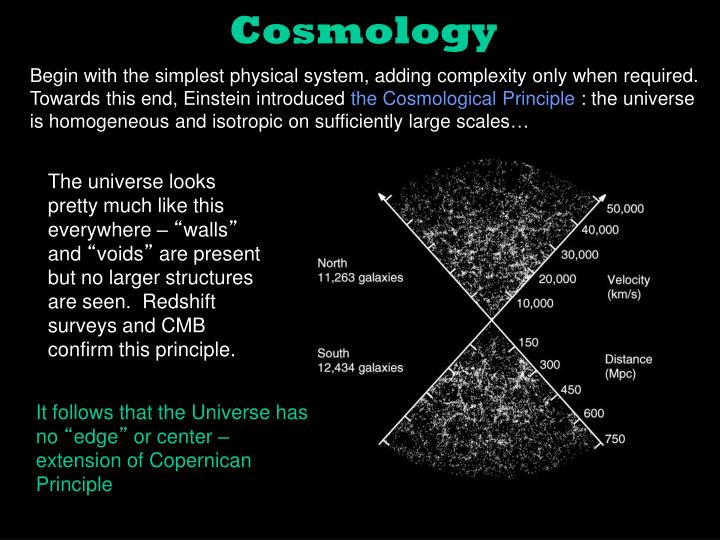
Cosmology Begin with the simplest physical system, adding complexity only when required. Towards this end, Einstein introduced the Cosmological Principle : the universe is homogeneous and isotropic on sufficiently large scales… The universe looks pretty much like this everywhere – “walls” and “voids” are present but no larger structures are seen. Redshift surveys and CMB confirm this principle. It follows that the Universe has no “edge” or center – extension of Copernican Principle
Hubble’s Law (Hubble 1929) the recessional velocity of external galaxies is linearly related to their distance. recession velocity = Ho x distance Derive Hubble’s law from the Cosmological Principle Consider a small triangle. As the universe expands or contracts, the conditions of homogeneity and isotropy require that the expansion is identical in all locations. The triangle must grow self-similarly. Define the present time at to and the scale factor of the expansion as a(t), with ao = a(to) being the scale factor at to. Self-similarity requires that any distance x increase by the same scale factor. Where Hubble parameter is Ho is value of the Hubble parameter at to Note that the Cosmological Principle does not require H > 0 – can have static or contracting universe.
Dynamics of the Universe - Conservation Laws and Friedmann Equations To solve for the dynamics of the universe, we will assume the Cosmological Principle along with General Relativity. Begin with a Newtonian approximation to derive the evolution of the universe. Use Lorentzian transformations within the Newtonian framework Approximate a region of the universe as a uniform density sphere of non-relativistic matter. Use the Eulerian equations (like CBE used for stars in galaxies!) for conservation of mass and momentum to derive the dynamical evolution of the universe. If mass is conserved, mass density satisfies EOC +
Time dependence is determined solely by the evolution of the scale factor - for a matter dominated Universe ρ ~ a-3
Apply conservation of momentum using Newton’s theory of gravity (though difficult to define potential in a uniform unbound medium like the Universe!). Apply Newton’s laws to a universe which is interior of large sphere (doesn’t violate CP badly if we consider only regions where x << Runiverse). Euler’s equation for momentum conservation or where v is the local fluid velocity, p is the pressure, and F is the force (in this case gravitational) per unit mass. If p gradient is zero (for CP) and x x = x, then, Using And mass conservation Universe must be changing velocity if it contains matter!
Einstein used GR to improve upon Newtonian cosmology and provide a description of the Universe as a whole. He introduced the cosmological constant Λ into his GR equations since he found (as we did) that if the density of the Universe is non-zero, the Universe must be expanding. As this was before Hubble’s work and most believed in a Steady State Universe, this constant allowed for a non-zero density and a static Universe. (After Hubble’s discovery of an expanding Universe, Einstein called this his “greatest blunder”.) Start with modification to Poisson’s law, Positive Λ is repulsive force that counteracts gravity. Now replace density with ρeff = ρ + 3p/c2 total energy density (kinetic + rest mass) GetFriedmann solutionsfor the scale factor of the Universe by multiplying by da/dt and integrating wrt time. For expanding Universe, gravitational term dominates when scale factor is small. At later times, first the curvature term then later the cosmological constant dominate.
Let’s work through one possible solution to the Friedmann equations with a simplicity assumption of a null cosmological constant, Λ = 0, and recall Evaluate the constant k in terms of present day observable quantities. k = 0 only when density is at the critical density, defined as Cosmological Density Parameter Inserting back into Friedmann equation we get
Case 1: k = 0 and Ωo= 1 Case 2: k > 0 and Ωo> 1 Case 3: k < 0 and Ωo< 1 Einstein-deSitter universe The Universe expands at an ever decreasing rate! Borderline Universe or Marginally Bound Energy term is now positive. Solution for a(t) is analogous to a rocket shot with velocity greater than escape velocity. Expansion continues forever! Open or Unbound Universe As scale factor increases, it eventually reaches a point where adot = 0. Expansion stops at amax. After amax is reached, Universe starts to collapse! Closed or Bound Universe
The Fate of the Universe Whether or not the universe continues to expand forever or eventually collapses depends on its density. High density = lots of mass = enough matter to gravitationally halt expansion and cause gravitational collapse Low density = little mass = not enough gravitational attraction to stop expansion…it goes on forever If Ho = 70 km/s/Mpc, then ρcrit ≈ 1 x 10-29 g/cm3 (about one H atom in 200 L volume of space)
Cosmology and General Relativity Einstein’s principle of equivalence led to the concept that space-time is curved in the presence of a gravitational field. The mass density of the Universe tells us about the geometry of space-time. Thus, we must interpret the solutions for the scale factor obtained from Newtonian theory within the framework of GR (Friedmann equations can be derived from Einstein’s field equations). Particles moving under the influence of gravity travel along geodesics, the shortest distance between two points in curved spacetime. k is positive or > 1, Bound/Closed Universe k is negative or < 1, Open Universe k = 0 or = 1, Flat/Marginally Bound/Critical Universe
Curvature is easily visualized with 2D analogy (creatures living on the surface of a sphere) • Detected by measuring the sum of the angles of any triangle • Locally, space may appear flat (Euclidean) • Define a metric along the surface • Ametric, or distance measure, describes the distance, ds, between two points in space or space-time ds2 = gijdxidxj • Ageodesicis the shortest distance between two points and can be found by minimizing the space or space-time interval, Metric for unit sphere Space-time metric: For special relativity, in a Lorentz frame we define a distance in spacetime as For light, the metric yields ds2 = 0. Light follows a null geodesic - meaning that the physical distance travelled is equal to ct. Everything that we see in the universe by definition lies along null geodesics, as the light has just had enough time to reach us.
3 Types of spacetime intervals: ds2 = zero - lightlike(photons travel along these lines - this is a lightcone in 2-d space) ds2 > zero - timelike(positions are close enough in space that a photon would have had more than enough time to travel from one event to the other) ds2 < zero - spacelike(photon cannot traverse the distance in the time given - one event could not have caused the other)
To construct a metric that is valid in a cosmological context, assume • the cosmological principle is true • each point in spacetime has one and only one co-moving, timelike geodesic passing through it • For a co-moving observer, there is a metric for the universe called the Robertson-Walker metric, or the Friedmann-LeMaitre-Robertson-Walker metric Where a is the scale factor of the Universe, r is the co-moving distance, k is the sign of curvature (0, -1, +1) and dη is the solid angle. This metric specifies the geometry of the universe with just one undetermined factor, a(t), which is determined from the Friedmann equations. Together, the Friedmann equations and RW metric completely describe the geometry. These are the co-moving coordinates of a point in space. If the expansion of the universe is homogeneous and isotropic, co-moving coordinates are constant with time. Co-moving distance DC = ro Proper distance DP = (a/ao)ro (Proper distance does change with time)
Cosmological Redshift We now have a means of describing the evolution of the size of the universe (Friedmann equation) and of measuring distances within the universe (Robertson-Walker metric). Recast these in terms of observable quantities we don’t directly observe a(t), but we can observe the cosmological redshift of objects due to the expansion of the universe. Recall the Doppler shift of light (redshift or blueshift) is defined as Since ao is a(to) then, ao=1 As Universe expands, photon’s λ expands proportionally to the scale factor a(t) Since redshift arises due to expanding wavelength of all photons traveling through an expanding Universe, it is called a cosmological redshift. As a consequence, we don’t normally convert redshift to distance, since we need to assume a particular model for how a(t) has evolved.
Friedmann equation in observable quantities Friedmann equation Critical value of Λ in flat, empty universe Recast F equation with these substitutions At time to Fundamental component of the Friedmann equation upon which our measures for the distance and evolution of other quantities will be based.
Expressing Distances in an Expanding Universe The geometry and expansion rate of the Universe effects angular sizes and distances measured. Integrate over components of RW metric. DH = c/Ho Hubble Distance (distance light travels in Hubble time, tH = 1/Ho) DC= Radial Co-moving Distance DM = sinhDC (-), DC (flat), sinDC (+) Transverse Co-moving Distance DA = L(proper length)/θ(angular size) = DM/(1+z) Angular Distance DL = sqrt (L/4π*flux) = DM(1+z) = DA(1+z)2 Luminosity Distance If Λ = 0 and flat geometry, then DL = 2c/Ho [z/(G+1)] {1+[z/(G+1)]} where G = (1 + z)1/2 See Ned Wright’s Javascript Cosmology Calculator for DL for different cosmologies: http://www.astro.ucla.edu/~wright/CosmoCalc.html
Angular Size vs Redshift As an object is moved to higher redshifts its angular size first decreases (as expected) but soon begins to increase after passing through a minimum value. The appearance of a minimum angular size at a given redshift zmin is a generic feature of cosmological models with Ωm > 0. Figure 10 from Sahni and Starobinsky (2000) The angular size as a function of cosmological redshift z for flat cosmological models ΩM+ΩΛ= 1. Heavier lines correspond to larger values of ΩM.
Luminosity distance vs z (plotting DL/DH) Angular diameter distance vs z (plotting DA/DH where DA=L/θ) DH=c/Ho= 3000h-1Mpc At high z, angular diameter distance is such that 1 arcsec is about 5 kpc. flat, Λ=0 – solid open, Λ=0 – dotted flat, non-zero Λ - dashed (from Hogg 2000 astro-ph 9905116)
Surface Brightness Dimming SB is flux per unit solid angle Recall Flux = L/(4πDL2)and the solid angle subtended by a source of projected area A is Ω = A/D2A Since DL = DA(1+z)2 we can show the surface brightness is Observed surface brightness of objects decreases very rapidly as one moves to high redshifts purely due to cosmology. Cosmological dimming is independent of cosmological parameters.
How does the age of the Universe differ in different cosmologies? Friedman models (Λ = 0) give to = (2/3)Ho-1 k = 0 0 < to < (2/3)Ho-1 k = +1 (2/3)Ho-1 < to < Ho-1 k = -1 What is the relationship between redshift and age of the Universe? Lookback time tL = 2/3Ho-1[1-(1+z)-3/2] for flat Universe Age of the Universe when light left source at redshift z te(Gyr) = 10.5 (Ho/65) (1+z)-3/2 for flat Universe
Lookback times vs z plotting tL/tH and age vs z plotting t/tH tL is difference between age of Universe now and age tU when photons left emitting source flat, Λ=0 – solid open, Λ=0 – dotted flat, non-zero Λ - dashed
Age of the Universe as calculated from various models. A flat universe with a significant cosmological constant (ΩM=0.3, ΩΛ=0.7) yields an age close to what you get with a constant value of Ho (tH or 1/Ho). 14 Age of ΩM=1, ΩΛ=0 universe is about 9 billion years Age of ΩM=0.3, ΩΛ=0.7 universe is about 14 billion years
Comparison of Different Cosmological Models qo is “deceleration parameter”
Classical Cosmological Tests (or How to determine if the Universe is Open, Closed, Flat or Accelerating?) 1) Add up all matter in the Universe to determine mass density Luminous matter: only ~1% of ρcrit Dark matter? Still a factor of ~5 to low to close the Universe with DM This only constrains ΩM and not the value of the cosmological constant ΩΛ which also impacts fate/age of the Universe From Big Bang Nucleosynthesis, we will see that baryonic matter is about 4-5% of the critical density with all matter (baryonic+DM) totaling ~30%.
2) Measure the curvature of space-time by surveying the Universe on large scales. Volume of space is a function of cosmological parameters. Thus, for a given class of objects the redshift distribution, N(z), will depend upon Ω0 (or ΩM) and ΩΛ. Assume a uniformly distributed population of objects with mean density n0. Then, Measurements attempted with QSO’s though important to remove evolutionary effects. Results indicate that if the Universe is curved, radius of curvature would have to be comparable to or greater than the Hubble distance – essentially flat…but why…. This is a challenge for Big Bang Cosmology
Models showing unbound, decelerating universe – more distant objects should be moving faster than nearby objects if the universe is decelerating. Objects were receding less rapidly in the past! 3) Look for dynamical effects on the expansion rate of the Universe (impacted by both ΩM and ΩΛ ). The rate of cosmic expansion can be determined by probing objects at great distances (several Gpc) where the geometry and Hubble parameter changes can be detected. Use Type 1 supernovae – standard candles that can be seen in distant galaxies (several Gpc) so galaxy distance can be determined independent from Universal expansion. 70 km/s/Mpc
Results from Type 1a Supernovae surveys Error ellipses show values consistent with best SNe data cosmological model fits Flatness criterion – dashed line d2a/dt2= 0 – solid diagonal Big Crunch below solid horizontal First evidence for accelerating Universal expansion