Download
1 / 45
450 likes | 560 Views
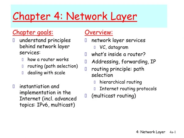
Chapter goals: understand principles behind network layer services: routing (path selection) dealing with scale how a router works advanced topics: IPv6, multicast instantiation and implementation in the Internet. Overview: network layer services routing principle: path selection

E N D
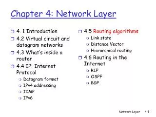
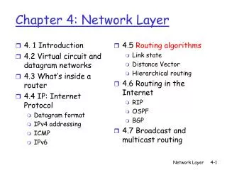
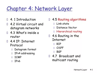
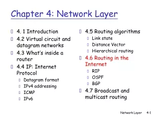
Chapter goals: understand principles behind network layer services: routing (path selection) dealing with scale how a router works advanced topics: IPv6, multicast instantiation and implementation in the Internet Overview: network layer services routing principle: path selection hierarchical routing IP Internet routing protocols reliable transfer intra-domain inter-domain what’s inside a router? IPv6 multicast routing Chapter 4: Network Layer 4: Network Layer
transport packet from sending to receiving hosts network layer protocols in every host, router three important functions: path determination: route taken by packets from source to dest. Routing algorithms switching: move packets from router’s input to appropriate router output call setup: some network architectures require router call setup along path before data flows network data link physical network data link physical network data link physical network data link physical network data link physical network data link physical network data link physical network data link physical application transport network data link physical application transport network data link physical Network layer functions 4: Network Layer
Q: What service model for “channel” transporting packets from sender to receiver? guaranteed bandwidth? preservation of inter-packet timing (no jitter)? loss-free delivery? in-order delivery? congestion feedback to sender? Network service model The most important abstraction provided by network layer: ? ? virtual circuit or datagram? ? service abstraction 4: Network Layer
call setup, teardown for each call before data can flow each packet carries VC identifier (not destination host OD) every router on source-dest path s maintain “state” for each passing connection transport-layer connection only involved two end systems link, router resources (bandwidth, buffers) may be allocated to VC to get circuit-like perf. “source-to-dest path behaves much like telephone circuit” performance-wise network actions along source-to-dest path Virtual circuits 4: Network Layer
used to setup, maintain teardown VC used in ATM, frame-relay, X.25 not used in today’s Internet application transport network data link physical application transport network data link physical Virtual circuits: signaling protocols 6. Receive data 5. Data flow begins 4. Call connected 3. Accept call 1. Initiate call 2. incoming call 4: Network Layer
no call setup at network layer routers: no state about end-to-end connections no network-level concept of “connection” packets typically routed using destination host ID packets between same source-dest pair may take different paths application transport network data link physical application transport network data link physical Datagram networks: the Internet model 1. Send data 2. Receive data 4: Network Layer
Network layer service models: Guarantees ? Network Architecture Internet ATM ATM ATM ATM Service Model best effort CBR VBR ABR UBR Congestion feedback no (inferred via loss) no congestion no congestion yes no Bandwidth none constant rate guaranteed rate guaranteed minimum none Loss no yes yes no no Order no yes yes yes yes Timing no yes yes no no • Internet model being extented: Intserv, Diffserv • Chapter 6 4: Network Layer
Internet data exchange among computers “elastic” service, no strict timing req. “smart” end systems (computers) can adapt, perform control, error recovery simple inside network, complexity at “edge” many link types different characteristics uniform service difficult ATM evolved from telephony human conversation: strict timing, reliability requirements need for guaranteed service “dumb” end systems telephones complexity inside network Datagram or VC network: why? 4: Network Layer
Graph abstraction for routing algorithms: graph nodes are routers graph edges are physical links link cost: delay, $ cost, or congestion level 5 3 5 2 2 1 3 1 2 1 A D B E F C Routing protocol Routing Goal: determine “good” path (sequence of routers) thru network from source to dest. • “good” path: • typically means minimum cost path • other def’s possible 4: Network Layer
Global or decentralized information? Global: all routers have complete topology, link cost info “link state” algorithms Decentralized: router knows physically-connected neighbors, link costs to neighbors iterative process of computation, exchange of info with neighbors “distance vector” algorithms Static or dynamic? Static: routes change slowly over time Dynamic: routes change more quickly periodic update in response to link cost changes Routing Algorithm classification 4: Network Layer
Dijkstra’s algorithm net topology, link costs known to all nodes accomplished via “link state broadcast” all nodes have same info computes least cost paths from one node (‘source”) to all other nodes gives routing table for that node iterative: after k iterations, know least cost path to k dest.’s Notation: c(i,j): link cost from node i to j. cost infinite if not direct neighbors D(v): current value of cost of path from source to dest. V p(v): predecessor node along path from source to v, that is next v N: set of nodes whose least cost path definitively known A Link-State Routing Algorithm 4: Network Layer
Dijsktra’s Algorithm 1 Initialization: 2 N = {A} 3 for all nodes v 4 if v adjacent to A 5 then D(v) = c(A,v) 6 else D(v) = infty 7 8 Loop 9 find w not in N such that D(w) is a minimum 10 add w to N 11 update D(v) for all v adjacent to w and not in N: 12 D(v) = min( D(v), D(w) + c(w,v) ) 13 /* new cost to v is either old cost to v or known 14 shortest path cost to w plus cost from w to v */ 15 until all nodes in N 4: Network Layer
5 3 5 2 2 1 3 1 2 1 A D B E F C Dijkstra’s algorithm: example D(B),p(B) 2,A 2,A 2,A D(D),p(D) 1,A D(C),p(C) 5,A 4,D 3,E 3,E D(E),p(E) infinity 2,D Step 0 1 2 3 4 5 start N A AD ADE ADEB ADEBC ADEBCF D(F),p(F) infinity infinity 4,E 4,E 4,E 4: Network Layer
Algorithm complexity: n nodes each iteration: need to check all nodes, w, not in N n*(n+1)/2 comparisons: O(n**2) more efficient implementations possible: O(nlogn) Oscillations possible: e.g., link cost = amount of carried traffic A A A A D D D D B B B B C C C C 2+e 2+e 0 0 1 1 1+e 1+e 0 e 0 0 Dijkstra’s algorithm, discussion 1 1+e 0 2+e 0 0 0 0 e 0 1 1+e 1 1 e … recompute … recompute routing … recompute initially 4: Network Layer
iterative: continues until no nodes exchange info. self-terminating: no “signal” to stop asynchronous: nodes need not exchange info/iterate in lock step! distributed: each node communicates only with directly-attached neighbors Distance Table data structure each node has its own row for each possible destination column for each directly-attached neighbor to node example: in node X, for dest. Y via neighbor Z: distance from X to Y, via Z as next hop X = D (Y,Z) Z c(X,Z) + min {D (Y,w)} = w Distance Vector Routing Algorithm 4: Network Layer
cost to destination via E D () A B C D A 1 7 6 4 B 14 8 9 11 D 5 5 4 2 1 7 2 8 1 destination 2 A D B E C E E E D (C,D) D (A,D) D (A,B) B D D c(E,B) + min {D (A,w)} c(E,D) + min {D (A,w)} c(E,D) + min {D (C,w)} = = = w w w = = = 2+3 = 5 2+2 = 4 8+6 = 14 Distance Table: example loop! loop! 4: Network Layer
cost to destination via E D () A B C D A 1 7 6 4 B 14 8 9 11 D 5 5 4 2 destination Distance table gives routing table Outgoing link to use, cost A B C D A,1 D,5 D,4 D,4 destination Routing table Distance table 4: Network Layer
Iterative, asynchronous: each local iteration caused by: local link cost change message from neighbor: its least cost path change from neighbor Distributed: each node notifies neighbors only when its least cost path to any destination changes neighbors then notify their neighbors if necessary wait for (change in local link cost of msg from neighbor) recompute distance table if least cost path to any dest has changed, notify neighbors Distance Vector Routing: overview Each node: 4: Network Layer
Distance Vector Algorithm: At all nodes, X: 1 Initialization: 2 for all adjacent nodes v: 3 D (*,v) = infty /* the * operator means "for all rows" */ 4 D (v,v) = c(X,v) 5 for all destinations, y 6 send min D (y,w) to each neighbor /* w over all X's neighbors */ X X X w 4: Network Layer
Distance Vector Algorithm (cont.): 8 loop 9 wait (until I see a link cost change to neighbor V 10 or until I receive update from neighbor V) 11 12 if (c(X,V) changes by d) 13 /* change cost to all dest's via neighbor v by d */ 14 /* note: d could be positive or negative */ 15 for all destinations y: D (y,V) = D (y,V) + d 16 17 else if (update received from V wrt destination Y) 18 /* shortest path from V to some Y has changed */ 19 /* V has sent a new value for its min DV(Y,w) */ 20 /* call this received new value is "newval" */ 21 for the single destination y: D (Y,V) = c(X,V) + newval 22 23 if we have a new min D (Y,w)for any destination Y 24 send new value of min D (Y,w) to all neighbors 25 26 forever X X w X X w X w 4: Network Layer
2 1 7 X Z Y Distance Vector Algorithm: example 4: Network Layer
2 1 7 Y Z X X c(X,Y) + min {D (Z,w)} c(X,Z) + min {D (Y,w)} D (Y,Z) D (Z,Y) = = w w = = 2+1 = 3 7+1 = 8 X Z Y Distance Vector Algorithm: example 4: Network Layer
1 4 1 50 X Z Y Distance Vector: link cost changes Link cost changes: • node detects local link cost change • updates distance table (line 15) • if cost change in least cost path, notify neighbors (lines 23,24) algorithm terminates “good news travels fast” 4: Network Layer
60 4 1 50 X Z Y Distance Vector: link cost changes Link cost changes: • good news travels fast • bad news travels slow - “count to infinity” problem! algorithm continues on! 4: Network Layer
60 4 1 50 X Z Y Distance Vector: poisoned reverse If Z routes through Y to get to X : • Z tells Y its (Z’s) distance to X is infinite (so Y won’t route to X via Z) • will this completely solve count to infinity problem? algorithm terminates 4: Network Layer
Message complexity LS: with n nodes, E links, O(nE) msgs sent each DV: exchange between neighbors only convergence time varies Speed of Convergence LS: O(n**2) algorithm requires O(nE) msgs may have oscillations DV: convergence time varies may be routing loops count-to-infinity problem Robustness: what happens if router malfunctions? LS: node can advertise incorrect link cost each node computes only its own table DV: DV node can advertise incorrect path cost each node’s table used by others error propagate thru network Comparison of LS and DV algorithms 4: Network Layer
scale: with 50 million destinations: can’t store all dest’s in routing tables! routing table exchange would swamp links! administrative autonomy internet = network of networks each network admin may want to control routing in its own network Hierarchical Routing Our routing study thus far - idealization • all routers identical • network “flat” … not true in practice 4: Network Layer
aggregate routers into regions, “autonomous systems” (AS) routers in same AS run same routing protocol “intra-AS” routing protocol routers in different AS can run different intra-AS routing protocol special routers in AS run intra-AS routing protocol with all other routers in AS also responsible for routing to destinations outside AS run inter-AS routing protocol with other gateway routers gateway routers Hierarchical Routing 4: Network Layer
c b b c a A.c A.a C.b B.a Intra-AS and Inter-AS routing • Gateways: • perform inter-AS routing amongst themselves • perform intra-AS routers with other routers in their AS b a a C B d A network layer inter-AS, intra-AS routing in gateway A.c link layer physical layer 4: Network Layer
Inter-AS routing between A and B b c a a C b B b c a d Host h1 A A.a A.c C.b B.a Intra-AS and Inter-AS routing Host h2 Intra-AS routing within AS B Intra-AS routing within AS A • We’ll examine specific inter-AS and intra-AS Internet routing protocols shortly 4: Network Layer
Host, router network layer functions: • ICMP protocol • error reporting • router “signaling” Transport layer: TCP, UDP • IP protocol • addressing conventions • datagram format • packet handling conventions • Routing protocols • path selection • RIP, OSPF, BGP Network layer routing table Link layer physical layer The Internet Network layer 4: Network Layer
IP address: 32-bit identifier for host, router interface interface: connection between host, router and physical link router’s typically have multiple interfaces host may have multiple interfaces IP addresses associated with interface, not host, router 223.1.1.2 223.1.1.1 223.1.2.2 223.1.2.1 223.1.3.2 223.1.3.1 223.1.3.27 223.1.2.9 223.1.1.4 223.1.1.3 223.1.1.1 = 11011111 00000001 00000001 00000001 223 1 1 1 IP Addressing: introduction 4: Network Layer
IP address: network part (high order bits) host part (low order bits) What’s a network ? (from IP address perspective) device interfaces with same network part of IP address can physically reach each other without intervening router IP Addressing 223.1.1.1 223.1.2.1 223.1.1.2 223.1.2.9 223.1.1.4 223.1.2.2 223.1.3.27 223.1.1.3 LAN 223.1.3.2 223.1.3.1 network consisting of 3 IP networks (for IP addresses starting with 223, first 24 bits are network address) 4: Network Layer
How to find the networks? Detach each interface from router, host create “islands of isolated networks 223.1.3.27 223.1.3.1 223.1.3.2 IP Addressing 223.1.1.2 223.1.1.1 223.1.1.4 223.1.1.3 223.1.7.0 223.1.9.2 223.1.9.1 223.1.7.1 223.1.8.1 223.1.8.0 223.1.2.6 Interconnected system consisting of six networks 223.1.2.1 223.1.2.2 4: Network Layer
multicast address 1110 network host 110 network 10 host IP Addresses given notion of “network”, let’s re-examine IP addresses: “class-full” addressing: class 1.0.0.0 to 127.255.255.255 A network 0 host 128.0.0.0 to 191.255.255.255 B 192.0.0.0 to 223.255.255.255 C 224.0.0.0 to 239.255.255.255 D 32 bits 4: Network Layer
host part network part 11001000 0001011100010000 00000000 200.23.16.0/23 IP addressing: CIDR • classful addressing: • inefficient use of address space, address space exhaustion • e.g., class B net allocated enough addresses for 65K hosts, even if only 2K hosts in that network • CIDR:Classless InterDomain Routing • network portion of address of arbitrary length • address format: a.b.c.d/x, where x is # bits in network portion of address 4: Network Layer
IP addresses: how to get one? Hosts (host portion): • hard-coded by system admin in a file • DHCP:Dynamic Host Configuration Protocol: dynamically get address: “plug-and-play” • host broadcasts “DHCP discover” msg • DHCP server responds with “DHCP offer” msg • host requests IP address: “DHCP request” msg • DHCP server sends address: “DHCP ack” msg 4: Network Layer
IP addresses: how to get one? Network (network portion): • get allocated portion of ISP’s address space: ISP's block 11001000 00010111 00010000 00000000 200.23.16.0/20 Organization 0 11001000 00010111 00010000 00000000 200.23.16.0/23 Organization 1 11001000 00010111 00010010 00000000 200.23.18.0/23 Organization 2 11001000 00010111 00010100 00000000 200.23.20.0/23 ... ….. …. …. Organization 7 11001000 00010111 00011110 00000000 200.23.30.0/23 4: Network Layer
200.23.16.0/23 200.23.18.0/23 200.23.30.0/23 200.23.20.0/23 . . . . . . Hierarchical addressing: route aggregation Hierarchical addressing allows efficient advertisement of routing information: Organization 0 Organization 1 “Send me anything with addresses beginning 200.23.16.0/20” Organization 2 Fly-By-Night-ISP Internet Organization 7 “Send me anything with addresses beginning 199.31.0.0/16” ISPs-R-Us 4: Network Layer
200.23.16.0/23 200.23.18.0/23 200.23.30.0/23 200.23.20.0/23 . . . . . . Hierarchical addressing: more specific routes ISPs-R-Us has a more specific route to Organization 1 Organization 0 “Send me anything with addresses beginning 200.23.16.0/20” Organization 2 Fly-By-Night-ISP Internet Organization 7 “Send me anything with addresses beginning 199.31.0.0/16 or 200.23.18.0/23” ISPs-R-Us Organization 1 4: Network Layer
IP addressing: the last word... Q: How does an ISP get block of addresses? A: ICANN: Internet Corporation for Assigned Names and Numbers • allocates addresses • manages DNS • assigns domain names, resolves disputes 4: Network Layer
IP datagram: 223.1.1.1 223.1.2.1 B E A 223.1.1.2 source IP addr 223.1.2.9 misc fields dest IP addr 223.1.1.4 data 223.1.2.2 223.1.3.27 223.1.1.3 223.1.3.2 223.1.3.1 Dest. Net. next router Nhops 223.1.1 1 223.1.2 223.1.1.4 2 223.1.3 223.1.1.4 2 Getting a datagram from source to dest. routing table in A • datagram remains unchanged, as it travels source to destination • addr fields of interest here 4: Network Layer
223.1.1.1 223.1.2.1 E B A 223.1.1.2 223.1.2.9 223.1.1.4 223.1.2.2 223.1.3.27 223.1.1.3 223.1.3.2 223.1.3.1 Dest. Net. next router Nhops 223.1.1 1 223.1.2 223.1.1.4 2 223.1.3 223.1.1.4 2 Getting a datagram from source to dest. misc fields data 223.1.1.1 223.1.1.3 Starting at A, given IP datagram addressed to B: • look up net. address of B • find B is on same net. as A • link layer will send datagram directly to B inside link-layer frame • B and A are directly connected 4: Network Layer
223.1.1.1 223.1.2.1 E B A 223.1.1.2 223.1.2.9 223.1.1.4 223.1.2.2 223.1.3.27 223.1.1.3 223.1.3.2 223.1.3.1 Dest. Net. next router Nhops 223.1.1 1 223.1.2 223.1.1.4 2 223.1.3 223.1.1.4 2 Getting a datagram from source to dest. misc fields data 223.1.1.1 223.1.2.3 Starting at A, dest. E: • look up network address of E • E on different network • A, E not directly attached • routing table: next hop router to E is 223.1.1.4 • link layer sends datagram to router 223.1.1.4 inside link-layer frame • datagram arrives at 223.1.1.4 • continued….. 4: Network Layer
Dest. next 223.1.1.1 network router Nhops interface 223.1.2.1 E B A 223.1.1 - 1 223.1.1.4 223.1.1.2 223.1.2 - 1 223.1.2.9 223.1.2.9 223.1.1.4 223.1.3 - 1 223.1.3.27 223.1.2.2 223.1.3.27 223.1.1.3 223.1.3.2 223.1.3.1 Getting a datagram from source to dest. misc fields data 223.1.1.1 223.1.2.3 Arriving at 223.1.4, destined for 223.1.2.2 • look up network address of E • E on same network as router’s interface 223.1.2.9 • router, E directly attached • link layer sends datagram to 223.1.2.2 inside link-layer frame via interface 223.1.2.9 • datagram arrives at 223.1.2.2!!! (hooray!) 4: Network Layer