Download
1 / 12
120 likes | 240 Views
CORIE circulation modeling system. Simulation databases. Daily forecasts. Codes: SELFE, ELCIRC 3D baroclinic Unstructured grids. Princeton Ocean Model (POM) (Mellor and Blumberg) Regional Ocean Modeling System, Haidvogel et al. (Rutgers Univ.)

E N D
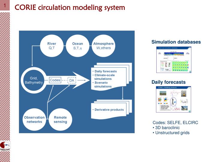
CORIE circulation modeling system Simulation databases Daily forecasts • Codes: SELFE, ELCIRC • 3D baroclinic • Unstructured grids
Princeton Ocean Model (POM) (Mellor and Blumberg) • Regional Ocean Modeling System, Haidvogel et al. (Rutgers Univ.) • Miami Isopycnic Model, Bleck et al. (University of Miami) • Modular Ocean Model, Bryan and Cox, GFDL • Finite Volume Community Ocean Model, C. Chen (University of Massacusetts) • Spectral Element Ocean Model, Levin et al. (Rutgers Univ.) 7. Advanced Circulation, Luettich et al. (Univ. of UNC, Waterway Experiment Station of Army Corp of Engineers):QUODDY, Lynch et al. (Dartmouth College) 8. Unstructured Tidal River Inter-tidal Mudflat, Casulli (Univ. of Trento, Italy); Eulerian-Lagrangian Circulation, Zhang, Baptista & Myers (OHSU) 9. Semi-implicit Eulerian-Lagrangian Finite Element, Zhang and Baptista (OHSU)
Introduction to governing equations Depth-averaged form: Continuity Salt and heat conservation
Introduction to governing equations Conservation of momentum (from Newton’s 2nd law: f=ma)
Introduction to governing equations Equation of state = (s, T, p) Turbulence closure equations
Adapted from Arun Chawla’s class notes for EBS575/675 Introduction to Fluid Dynamics Conservation of mass - water Consider a control volume of infinitesimal size dz dy dx Let density = Let velocity = Mass inside volume = Mass flux into the control volume = Mass flux out of the control volume =
Adapted from Arun Chawla’s class notes for EBS575/675 Introduction to Fluid Dynamics Conservation of mass Conservation of mass states that Rate of change of mass inside the system = Mass flux into of the system – Mass flux out the system Thus and, after differentiation by parts
Adapted from Arun Chawla’s class notes for EBS575/675 Introduction to Fluid Dynamics Conservation of mass Rearranging, For incompressible fluids, like water and, thus
Adapted from Arun Chawla’s class notes for EBS575/675 Introduction to Fluid Dynamics Conservation of mass of a solute Let flux of mass per unit area entering the system = Let flux of mass per unit area leaving the system = Consider a 1D system with stationary fluid and a solute that is diffusing dy dx Let concentration (mass /unit volume) of solute inside the control volume = C
Adapted from Arun Chawla’s class notes for EBS575/675 Introduction to Fluid Dynamics Conservation of mass of a solute Mass flux of solute leaving the system – mass flux of solute entering the system = rate of change of solute in the system Conservation of mass states that Thus or
Adapted from Arun Chawla’s class notes for EBS575/675 Introduction to Fluid Dynamics Conservation of mass of a solute How do we quantify q ? • In a static fluid, flux of concentration (q), occurs due to random molecular motion • It is not feasible to reproduce molecular motion on a large scale. • Thus, we wish to represent the molecular motion by the macroscpoic property of the solute (its concentration, C) Also, from observation we know • In a fluid of constant C (well mixed liquid), there is no net flux of concentration • Solute moves from a region of high concentration to regions of low concentration • Over some finite time scale, the solute does not show any preferential direction of motion
Adapted from Arun Chawla’s class notes for EBS575/675 Introduction to Fluid Dynamics Conservation of mass of a solute Diffusion coefficient Fick’s law Based on these observations, Adolph Fick (1855) hypothesized that (molecular processes are represented by an empirical coefficient analogous to viscosity) or in three dimensions Applying Fick’s law to the 1D mass conservation equation for a solute, we get or