Download
1 / 25
250 likes | 350 Views
Discover the importance of defining trajectory similarity for data analysis tasks with LCSS, p-norm, and time-warping techniques. Explore indexing structures, accuracy experiments, and related work. Conclusion highlights efficient algorithms.

E N D
Discovering Similar Multidimensional Trajectories ICDE, San Jose, CA, 2002
Outline • Introduction • Similarity Measures • Compute the Similarity • Indexing Trajectories • Experimental Evaluation • Related Work • Conclusion
Introduction • The trajectory of a moving object is typically modeled as a sequence of consecutive locations in a multidimensional Euclidean space • An appropriate and efficient model for defining the similarity for trajectory data will be very important for the quality of the data analysis tasks.
Hierarchical clustering of 2D series (displayed as 1D for clariry)
Similarity Measures • Let A and Bbe two trajectories of moving objects with size n and mrespectively, where A = ((ax,1 , ay,1),…,(ax,n , ay,n)) and B = ((bx,1, by,1),…,(bx,m, by,m)). For a trajectory A, let Head(A) be the sequence Head(A) = ((ax,1, ay,1),…,(ax,n-1, ay,n-1))
Definition 1 • Given an integer δand a real number 0 < ε <1, we define the LCSSδ,ε(A; B) as follows:
Definition 2 • We define the similarity function S1 between two trajectories A and B, given δ and ε, as follows:
Definition 3 • Given δ, εand the family Fof translations, we define the similarity function S2 between two trajectories A and B, as follows:
Definition 4 • Given δ,εand two trajectories A and B we define the following distance functions:
Compute the Similarity • Similarity function S1 • Given two trajectories A and B, with |A| = n and |B| = m, we can find the LCSSδ,ε(A, B) in O(δ(n + m)) time. • Similarity function S2 • Given two trajectories A and B, with |A| = n and |B| = m, we can compute the S2(δ,ε, A, B) in O((n+m)3δ3) time.
Indexing Structure • For every node C of the tree we store the medoid (MC) of each cluster. The medoid is the trajectory that has the minimum distance (or maximum LCSS) from every other trajectory in the cluster:
Time and Accuracy Experiments • Similarity values and running times from SEALS dataset
Related Work • Use a p-norm distance to define the similarity measure. [2, 37, 18, 14, 10, 32, 10, 20, 24, 23] • Based on the time warping technique.[5, 25, 28, 33] • Find the longest common subsequence (LCSS) of two sequences.[3, 7, 11] • Define time series similarity are based on extracting certain features.[13, 17, 29, 31]
Conclusion • Efficient techniques to accurately compute the similarity between trajectories • Approximate algorithms with provable performance bounds • efficient index structure
Comments • Good approach for similarity queries • Use real GPS trajectory data? • …
Dynamic Time Warping • Sequences are similar but accelerate differently along the time axis • Enforcing a temporal constraint δ on the warping window size improves computation efficiency and accuracy • Application: Speech recognition (Berndt and Clifford, 1996)
Longest Common Subsequence Similarity • Match 2 sequences by allowing some elements to be unmatched • C = {1,2,3,4,5,1,7} and Q = {2,5,4,5,3,1,8} • Longest is {2,4,5,1} • Application: Bioinformatics 2 5 4 5 3 1 8 1 2 3 4 5 1 7 0 0 0 0 1 0 1 1 1 1 1 1 1 1 1 2 2 2 1 1 1 1 2 2 2 2 2 1 1 3 3 2 2 3 3 1 3 3 2 2 4 4 Dissimilarity: 1 3 3 2 2 4 4 2 1 4 5 Tolerance: c Vlachos et al., 2002
Longest Common Subsequence Similarity • Input sequences C[1..m] and Q[1..n] • Compute LCS btwn C[1..i] and Q[1..j] • for all 1 ≤ i ≤ m and 1 ≤ j ≤ n • Stores it in L[i,j] • L[m,n] = length of the LCS 2 5 4 5 3 1 8 1 2 3 4 5 1 7 0 0 0 0 1 0 1 1 1 1 1 1 1 1 1 2 2 2 1 1 1 1 2 2 2 for i := 1..m for j := 1..n if C[i] = Q[j] L[i,j] := L[i-1,j-1] + 1 • else: • L[i,j] := max(L[i,j-1], L[i-1,j]) return L[m,n] 2 2 1 1 3 3 2 2 3 3 1 3 3 2 2 4 4 1 3 3 2 2 4 4 2 1 4 5 Vlachos et al., 2002