Download
1 / 18
180 likes | 299 Views
The Paradigm of Optoelectronics. optics. experiment medium, or optical circuit. optical SOURCE. DETECTOR. signal out. signal in. information. processing. optoelectronics. electronics. a good photodetector is like a good source. P. received. S/N = (atten) P / P.

E N D
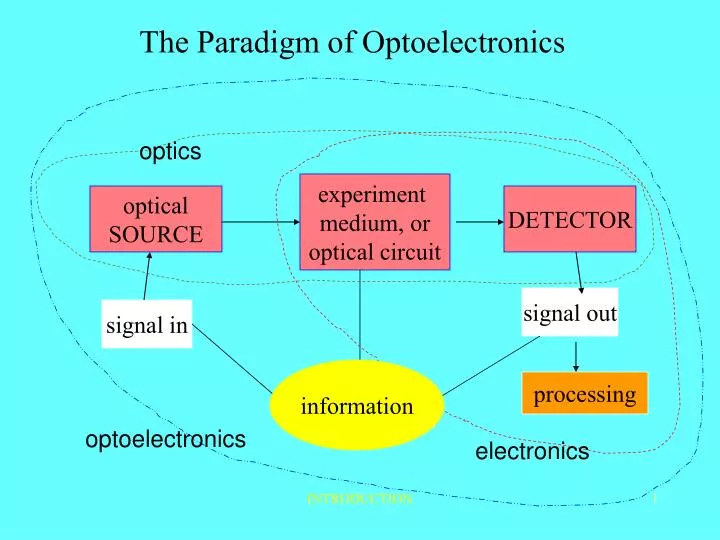
The Paradigm of Optoelectronics optics experiment medium, or optical circuit optical SOURCE DETECTOR signal out signal in information processing optoelectronics electronics INTRODUCTION
a good photodetector is like a good source P received S/N = (atten) P / P . source noise decreasing detector noise by K is the same as increasing source power by K .!.! system quality factor INTRODUCTION
Milestones in Photodetection 1829-33: Nobili(I) and Macedonio Melloni (I) invent the thermopile 1873: W. Smith (UK) discovers photoconductivity in Selenium 1905: A.Einstein explains photoemission by the quanta hypotesis 1910s: first S-1 photocathodes and vacuum-photodiodes 1919: J. Slepian (USA) invents the photomultiplier 1930: V. Zworikyn and G. Morton (USA) demonstrate television 1930: Image converter tubes and streak-camera tubes developed 1940s: The ‘Sniperscope’ image converter tubes used as night-vision aid 1950s: Solid-state theory developed, first Ge-photodiodes 1965: Planar Si-photodiodes, EBS camera tubes, InSb IR-detectors 1967: Apollo 11 send images of the moon taken with EBS 1967: Avalanche photodiodes invented 1970: first CCD image-pickup devices 1970: The Apollo 15 Lunar Ranging Experiment 1975: Compound semiconductor photodiodes cover all the IR bands 1980: Camcorders with CCDs are mass produced 1995: room-temperature Thermovisions 1996: Hubble Space Telescope is equipped with a CCD camera INTRODUCTION
Photodetectors and their Spectral Ranges • SINGLE ELEMENT IMAGE • - photoemission devices vacuum photodiode pickup tubes • (or external gas photodiode image intensifiers • photoelectric devices) photomultiplier and converters • - internalphotoelectric semiconductor photodiode CCDs • devices avalanche photodiode • phototransistor (BJT, FET) • photoresistance vidicon • - thermal detectors thermocouple (or photopile) • thermistor (or bolometer) uncooled IR FPA • pyroelectric IR vidicon • - weak interaction photon drag, Golay cell • detectors photoelectromagnetic • point contact diode • 0.1mm 1mm 10mm 100mm (l) • ___|_____________|_____________|_____________|_____________|_ • __photoemission ____ • ____internal photoelectric effect _____ • _____________________thermal________________________________
Detectors based on Photoelectric effect Power collected P = hn F is a flux F of photons of energy hn Output current I =e F’ is a flux F’ of electrons of charge e Then, current is proportional to power, I/P= s = e F’ / hn F = h (e /hn) where h = F’/F is quantum efficiency (electrons-to-photons) and s = I/P= h (le /hc) = h(l/1.24) [A/W] is spectral sensitivity (current out -to-power in) INTRODUCTION
Detectors based on Photoelectric effect 2 To trade photons for electrons we need a material requiring an energy not larger than the photon energy, so hn≥Ecc , where energy Ecc for the charge carrier generation is EW(work function) in external and EG(bandgap) in internal photoemission. This is the threshold condition: hc/l≥Ecc or l ≤ lt = hc/eEcc = 1.24 / Ecc(eV) In alkaline antimonides, EW ≈1.2-3.0 eV, and lt ≈1-0.4 mm (blue to NIR) ternaries (InGaAs) EG ≈0.75 eV, lt ≈1.8 mm InSb EG ≈0.25 eV, lt ≈5 mm (MIR) HgCdTe EG ≈0.08 eV, lt ≈16 mm (FIR) INTRODUCTION
Detectors based on Photoelectric effect 3 general response curve of a quantum detector: at P=cons, current increases linearly with l, then sharply decreases to 0 at the photoelectric threshold a real detector has a curve rather than a triangle INTRODUCTION
Detectors based on Photoelectric effect 4 Once produced, we shall remove charge carriers fast, so we need very thin layers to cross or a favorable electric field helping collection photocathodes pn junction in a diode base-collector junct.of BJT gate-drain junct in a FET depleted layer in a MOS 3rd junct in a SCR applied field in a resistance INTRODUCTION
(S/N) √Iph0/2eB I / I ph ph0 Quantum detectors: S/N vs Iph 2 10 170 10 dB/dec 10 160 quantum regime with noise factor F S/N (dB re 1mA,1Hz) 1 F 150 20 dB/dec -1 10 140 thermal regime -2 quantum regime 10 130 -1 3 -2 2 1 10 10 10 10 10 INTRODUCTION
Time measurements - best with n=12 stages (G=107 - 108) for weak signals - output terminated on Rc=50 W for best bandwidth, first (3R) and last dynodes with more voltage (3R, 6R) impulse response: SER-limited (typ. duration Dt =2 ns), intrinsic limit of accuracy: sT={st02+[g/(g-1)g1]sti2}1/2 (typ.)=0.58 ns for 1 photoelectron PMT APPLICATIONS
Time measurements Time resolution of a typical 12-stage PMT with Dt=3 ns followed by a constant fraction timing (CFT). Data for a I(t)=d(t) light pulse; timing threshold is set at a fractional level S0 =C/R of the total collected charge R. PMT APPLICATIONS
Photon counting basic functional scheme of photon counting with PMTs (top), and an example of a measurement, showing evolution of signal plus dark, dark only, and result after dark subtraction (bottom); vertical bars on DN indicate the ±0.5sDn standard deviation confidence intervals PMT APPLICATIONS
Photon counting (cont’d) • Requirements for PMTs in a photocounting regime: • a SER amplitude in the mA range (to get ≈100mV in circuits), i.e., G≈107-108 and n≈12 dynodes • a high first dynode gain for a good discrimination efficiency • a voltage divider adequate to have a short Dtof SER. • - maximum photon rate acquired for the photocounting: • F=1/Tr (set by the integrator recovery time, Tr =3-10 Dt typ. ) • - dynamic range (in power): • P=e/Trs (for s=20mA/W, Tr=10ns it is P=0.8 nW) PMT APPLICATIONS
Analysis of the photon counting Total counting N= Ns+Nd, (signal plus dark) has a mean value: áNñ= áNsñ+áNdñ = h.hp F T +(hdId /e)T and, following Poisson statistics, variance is: sN2 = áNsñ+ áNdñ whence (S/N)2 = áNsñ2 / [áNsñ+áNdñ] noise figure NF2 of the photocounting process: NF2 = (S/N)2Nd=0/(S/N)2 =1+ áNdñ/áNsñ= 1+ (hdId /e)/h.hp F The minimum measurable radiant power, at dark counting rates Id/e of a few electrons/cm2.s, (at h. h p=0.1, near the peak of photocathode response) is: P = Fhn/h.hp »10-18 W a performance unsurpassed by any other kind of photodetector PMT APPLICATIONS
Photon counting with dark subtraction Subtracting dark from signal plus dark (with the same T)gives: DN= áN1ñ-áN2ñ=áNsñ+áNdñ-áNdñ=áNsñ The variance of DN is the sum of the variances, so that: sDN2 = áNsñ+2áNdñ (S/N)2 =áNsñ2/ [áNsñ+2áNdñ] and NF2 = 1+ 2áNdñ/áNsñ = 1+ (2hdId /e)/h.hp F letting S/N=1 and for weak signals (áNsñ<<áNdñ), it is: áNsñmin = √[2áNdñ] = √(2hdId T/e) or, the minimum detectable signal, being áNsñ=hhp FT, is: Fmin = √(2hdId /eT)/hhp PMT APPLICATIONS
Photon counting with dark subtraction: an example With a PMT having: - a S-24 response, with h=0.35 at l=400nm, - a 1cm2 area, with a dark current rate Id/e=1cm-2 - a first dynode gain g1=3 - thresholds Q1/Ge=0.8 and Q2/Ge=2.5 (hp=0.7, hd=0.8) the minimum detectable rate is: Fmin=√(2.0.7.1/T)/0.35.0.7 =4.83/√T photon/s. for a 8-hour integration period this yields: Fmin=4.83/√28800=0.028 photon/s, or Pmin=hnFmin= 1.3 .10-20 W, i.e., the power collected from a m= 28th magnitude star with a 1m2 telescope aperture. PMT APPLICATIONS
Nuclear spectrometry with scintillation counters functional scheme of energy spectrometry measurements (top) and waveforms (middle). The typical energy spectrum obtained with the scintillation detector (bottom) reveals radionuclides species (energy signature) and their concentrations (counts intensity) PMT APPLICATIONS
Dating with scintillation counters Carbon isotope 14C, initially absorbed from atmosphere during specimen life, decays with a half-life T1/2=5700 years emitting 160 keV electrons. Dating is performed by looking at the detection rate of 160 keV electrons (peak amplitude of the MCA+scintillator spectrum), which is proportional to the residual content of 14C in it. Measurable concentrations are down to c=10-3 of the initial value c0, according to the simple expression T=T1/2 log2 (c/c0), with a practical limit in dating to about 40 000 years. Other radionuclides, such as 87Rb, 232Th, 235U and 40K, are used to cover much larger time spans (up to 106-109 years) and in inorganic samples where 14C is absent PMT APPLICATIONS