Download
1 / 42
430 likes | 612 Views
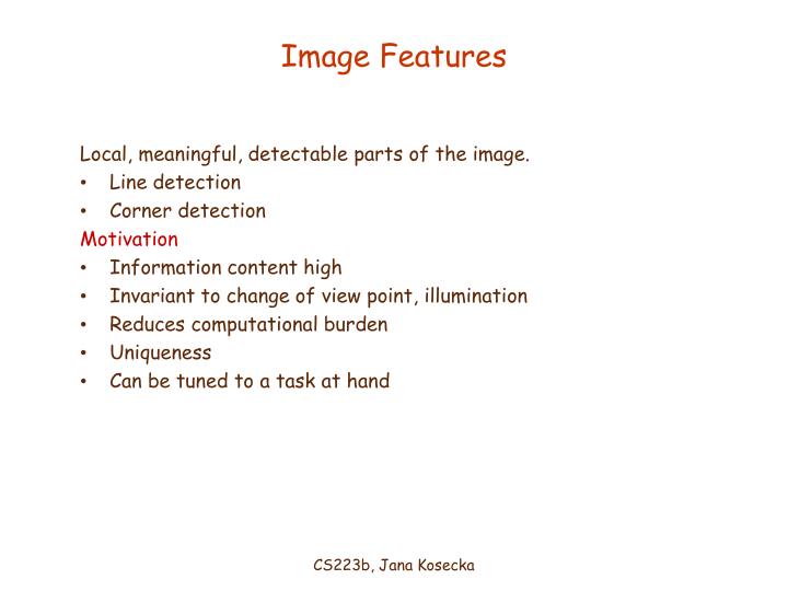
Image Features. Local, meaningful, detectable parts of the image. Line detection Corner detection Motivation Information content high Invariant to change of view point, illumination Reduces computational burden Uniqueness Can be tuned to a task at hand. Canne Edge Detector. Before:.

E N D
Image Features Local, meaningful, detectable parts of the image. • Line detection • Corner detection Motivation • Information content high • Invariant to change of view point, illumination • Reduces computational burden • Uniqueness • Can be tuned to a task at hand CS223b, Jana Kosecka
Canne Edge Detector Before: • Edge detection involves 3 steps: • Noise smoothing • Edge enhancement • Edge localization • J. Canny formalized these steps to design an optimaledge detector • How to go from derivatives to edges ? Horizontal edges CS223b, Jana Kosecka
Edge Detection original image gradient magnitude Canny edge detector • Compute image derivatives • if gradient magnitude > and the value is a local maximum along gradient • direction – pixel is an edge candidate CS223b, Jana Kosecka
Algorithm Canny Edge detector • The input is image I; G is a zero mean Gaussian filter (std = ) • J = I * G (smoothing) • For each pixel (i,j): (edge enhancement) • Compute the image gradient • J(i,j) = (Jx(i,j),Jy(i,j))’ • Estimate edge strength • es(i,j) = (Jx2(i,j)+ Jy2(i,j))1/2 • Estimate edge orientation • eo(i,j) = arctan(Jx(i,j)/Jy(i,j)) • The output are images Es - Edge Strength - Magnitude • and Edge Orientation Eo - CS223b, Jana Kosecka
Th • Es has large values at edges: Find local maxima • … but it also may have wide ridges around the local maxima (large values around the edges) CS223b, Jana Kosecka
NONMAX_SUPRESSION Edge orientation • The inputs are Es& Eo(outputs of CANNY_ENHANCER) • Consider 4 directions D={ 0,45,90,135} wrt x • For each pixel (i,j) do: • Find the direction dD s.t. d Eo(i,j) (normal to the edge) • If {Es(i,j) is smaller than at least one of its neigh. along d} • IN(i,j)=0 • Otherwise, IN(i,j)= Es(i,j) • The output is the thinned edge image IN CS223b, Jana Kosecka
Graphical Interpretation x x CS223b, Jana Kosecka
Thresholding • Edges are found by thresholding the output of NONMAX_SUPRESSION • If the threshold is too high: • Very few (none) edges • High MISDETECTIONS, many gaps • If the threshold is too low: • Too many (all pixels) edges • High FALSE POSITIVES, many extra edges CS223b, Jana Kosecka
SOLUTION: Hysteresis Thresholding Es(i,j)>L Es(i,j)<H Es(i,j)> H Es(i,j)<L Es(i,j)>L CS223b, Jana Kosecka
gap is gone Canny Edge Detection (Example) Strong + connected weak edges Original image Strong edges only Weak edges courtesy of G. Loy CS223b, Jana Kosecka
Other Edge Detectors (2nd order derivative filters) CS223b, Jana Kosecka
F ’(x) F(x) x First-order derivative filters (1D) • Sharp changes in gray level of the input image correspond to “peaks” of the first-derivative of the input signal. CS223b, Jana Kosecka
F’’(x) F ’(x) F(x) x Second-order derivative filters (1D) • Peaks of the first-derivative of the input signal, correspond to “zero-crossings” of the second-derivative of the input signal. CS223b, Jana Kosecka
NOTE: • F’’(x)=0 is not enough! • F’(x) = c has F’’(x) = 0, but there is no edge • The second-derivative must change sign, -- i.e. from (+) to (-) or from (-) to (+) • The sign transition depends on the intensity change of the image – i.e. from dark to bright or vice versa. CS223b, Jana Kosecka
y F(x) x x dI(x) d2I(x) > Th dx dx2 = 0 2I(x,y) =Ix x (x,y) + Iyy (x,y)=0 |I(x,y)| =(Ix 2(x,y) + Iy2(x,y))1/2 > Th tan = Ix(x,y)/ Iy(x,y) Laplacian Edge Detection (2D) 1D 2D I(x) I(x,y) CS223b, Jana Kosecka
Notes about the Laplacian: • 2I(x,y) is a SCALAR • Can be found using a SINGLE mask • Orientation information is lost • 2I(x,y) is the sum of SECOND-order derivatives • But taking derivatives increases noise • Very noise sensitive! • It is always combined with a smoothing operation: CS223b, Jana Kosecka
LOG Filter • First smooth (Gaussian filter), • Then, find zero-crossings (Laplacian filter): • O(x,y) = 2(I(x,y) * G(x,y)) • Using linearity: • O(x,y) = 2G(x,y) * I(x,y) • This filter is called: “Laplacian of the Gaussian” (LOG) CS223b, Jana Kosecka
1D Gaussian CS223b, Jana Kosecka
First Derivative of a Gaussian Positive Negative As a mask, it is also computing a difference (derivative) CS223b, Jana Kosecka
2D Second Derivative of a Gaussian “Mexican Hat” CS223b, Jana Kosecka
An edge is not a line... • How can we detect lines ? CS223b, Jana Kosecka
Finding lines in an image • Option 1: • Search for the line at every possible position/orientation • What is the cost of this operation? • Option 2: • Use a voting scheme: Hough transform CS223b, Jana Kosecka
Finding lines in an image y b • Connection between image (x,y) and Hough (m,b) spaces • A line in the image corresponds to a point in Hough space • To go from image space to Hough space: • given a set of points (x,y), find all (m,b) such that y = mx + b b0 m0 x m image space Hough space CS223b, Jana Kosecka
Finding lines in an image y b • Connection between image (x,y) and Hough (m,b) spaces • A line in the image corresponds to a point in Hough space • To go from image space to Hough space: • given a set of points (x,y), find all (m,b) such that y = mx + b • What does a point (x0, y0) in the image space map to? y0 x0 x m image space Hough space • A: the solutions of b = -x0m + y0 • this is a line in Hough space CS223b, Jana Kosecka
Hough transform algorithm • Typically use a different parameterization • d is the perpendicular distance from the line to the origin • is the angle this perpendicular makes with the x axis • Why? Idea – keep an accumulator array (Hough space) and let each edge pixel contribute to it Line candidates are the maxima in the accumulator array CS223b, Jana Kosecka
Typical Hough Transform • Basic Hough transform algorithm • 1. Initialize H[d, q]=0 • 2. For each edge point I[x,y] in the image • 3. For q = 0 to 180 • H[d, q] += 1 where • point is now a sinusoid in Hough space • Find the value(s) of (d, q) where H[d, q] is maximum • The detected line in the image is given b • What’s the running time (measured in # votes)? CS223b, Jana Kosecka
Radon transform CS223b, Jana Kosecka
Hough Transform for Curves • The H.T. can be generalized to detect any curve that can be expressed in parametric form: • Y = f(x, a1,a2,…ap) • a1, a2, … ap are the parameters • The parameter space is p-dimensional • The accumulating array is LARGE! CS223b, Jana Kosecka
y x Line fitting Non-max suppressed gradient magnitude • Edge detection, non-maximum suppression • (traditionally Hough Transform – issues of resolution, threshold • selection and search for peaks in Hough space) • Connected components on edge pixels with similar orientation • - group pixels with common orientation CS223b, Jana Kosecka
Line Fitting second moment matrix associated with each connected component v1 - eigenvector of A • Line fitting lines determined from eigenvalues and eigenvectors of A • Candidate line segments - associated line quality CS223b, Jana Kosecka
Corners contain more edges than lines. Corner detection • A point on a line is hard to match. CS223b, Jana Kosecka
Finding Corners • Intuition: • Right at corner, gradient is ill defined. • Near corner, gradient has two different values. CS223b, Jana Kosecka
Formula for Finding Corners We look at matrix: Gradient with respect to x, times gradient with respect to y Sum over a small region, the hypothetical corner Matrix is symmetric CS223b, Jana Kosecka
First, consider case where: • This means all gradients in neighborhood are: • (k,0) or (0, c) or (0, 0) (or off-diagonals cancel). • What is region like if: • l1 = 0? • l2 = 0? • l1 = 0 and l2 = 0? • l1 > 0 and l2 > 0? CS223b, Jana Kosecka
General Case: From Linear Algebra, it follows that because C is symmetric: With R a rotation matrix. So every case is like one on last slide. CS223b, Jana Kosecka
So, to detect corners • Filter image. • Compute magnitude of the gradient everywhere. • We construct C in a window. • Use Linear Algebra to find l1 and l2. • If they are both big, we have a corner. CS223b, Jana Kosecka
Point Feature Extraction • Compute eigenvalues of G • If smalest eigenvalue of G is bigger than - mark pixel as candidate • feature point • Alternatively feature quality function (Harris Corner Detector) CS223b, Jana Kosecka
% Harris Corner detector - by Kashif Shahzad sigma=2; thresh=0.1; sze=11; disp=0; % Derivative masks dy = [-1 0 1; -1 0 1; -1 0 1]; dx = dy'; %dx is the transpose matrix of dy % Ix and Iy are the horizontal and vertical edges of image Ix = conv2(bw, dx, 'same'); Iy = conv2(bw, dy, 'same'); % Calculating the gradient of the image Ix and Iy g = fspecial('gaussian',max(1,fix(6*sigma)), sigma); Ix2 = conv2(Ix.^2, g, 'same'); % Smoothed squared image derivatives Iy2 = conv2(Iy.^2, g, 'same'); Ixy = conv2(Ix.*Iy, g, 'same'); % My preferred measure according to research paper cornerness = (Ix2.*Iy2 - Ixy.^2)./(Ix2 + Iy2 + eps); % We should perform nonmaximal suppression and threshold mx = ordfilt2(cornerness,sze^2,ones(sze)); % Grey-scale dilate cornerness = (cornerness==mx)&(cornerness>thresh); % Find maxima [rws,cols] = find(cornerness); clf ; imshow(bw); hold on; p=[cols rws]; plot(p(:,1),p(:,2),'or'); title('\bf Harris Corners') CS223b, Jana Kosecka
Example (s=0.1) CS223b, Jana Kosecka
Example (s=0.01) CS223b, Jana Kosecka
Example (s=0.001) CS223b, Jana Kosecka
Harris Corner Detector - Example CS223b, Jana Kosecka