Download
1 / 30
320 likes | 676 Views
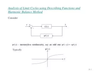
3-D Unsteady Multi-stage Turbomachinery Simulations using the Harmonic Balance Technique. Arti K. Gopinath, Edwin van der Weide, Juan J. Alonso, Antony Jameson Stanford University, CA Advanced Simulation and Computing (ASC) Program – DoE Kivanc Ekici and Kenneth C. Hall Duke University, NC.

E N D
3-D Unsteady Multi-stage Turbomachinery Simulations using the Harmonic Balance Technique Arti K. Gopinath, Edwin van der Weide, Juan J. Alonso, Antony Jameson Stanford University, CA Advanced Simulation and Computing (ASC) Program – DoE Kivanc Ekici and Kenneth C. Hall Duke University, NC
interface interface SUmb (URANS) CDP (LES) SUmb Stanford ASC Project combustor turbine compressor
Practical Turbomachinery: PW6000 5-stage HPC with 220 M cells => 2.4 M CPU hours
Mixing Plane Approximation • Steady computation in each blade row . • Computational grid spanning one blade passage per blade row • Circumferentially averaged quantities passed between blade rows • All unsteady effects lost
Time Dependent Calculations The URANS equations are semi-discretized as Time Derivative Term Solve in pseudo-time t* to its steady state Use standard convergence acceleration techniques: Runge-Kutta time stepping schemes with local Δt* Multigrid in space
Time Integration Methods: Backward Difference Formula(BDF) • General time integration method: • not specific for periodic problems • Periodic state reached after 4-6 • revolutions for high RPM cases • Transients take up most of the • resources. • Could be very expensive for • multi-stage turbomachinery
Time Integration Methods: Periodic Problems • Time Spectral method( time-domain method) and Frequency Domain methods. • Fourier Representation in Time • Full matrix => Solution at time instance n depends • on the solution of all other time instances Very expensive if high frequency unsteadiness need to be resolved
NASA Stage 35 Compressor 36 Rotors - 46 Stators Approximations and Reduced-Order Models .
Approximations and Reduced-Order Models . NASA Stage 35 Compressor Half Wheel 36 Rotors - 46 Stators 18 Rotors - 23 Stators Periodic Boundary Conditions Time Span = Time for Half Revolution
36 Rotors - 46 Stators scaled to 36 Rotors - 48 Stators reduced to periodic sector Computational Grid: 3 Rotors - 4 Stators Approximations and Reduced-Order Models Scaled NASA Stage 35 Compressor . Periodic Boundary Conditions Time Span = Time for Periodic Sector Often used with BDF and Time Spectral Method to keep costs low Solve an Approximate Problem
Approximations and Reduced-Order Models Harmonic Balance Technique . NASA Stage 35 Compressor True Geometry 36 Rotors - 46 Stators Computational Grid: 1 Rotor - 1 Stator Modified Periodic Boundary Conditions Time Span such that only dominant frequencies are resolved • Fraction of the cost of a BDF/Time Spectral Computation on the true geometry
Rotor Stator Rotor Stator2 Stator1 Blade Passing Frequency (BPF) Multi-Stage Case: Single-Stage Case: Combinations of BPF of Stator1 and Stator2 resolved in the Rotor row BPF of the Stator and its higher harmonics resolved in the Rotor row . BPF of the Rotor and its higher harmonics resolved in the Stator row Only BPF of Rotor resolved in Stator1 and Stator2 Only One Fundamental Frequency in each blade row No one fundamental frequency resolved by the rotor row
Savings in space: phase-lagged conditions . Phase-Lagged Boundary Conditions Periodic Boundary Conditions A A B B UA(t) = UB(t) UA(t) = UB(t-dt)
Savings in time:Smaller Time Span and only Dominant Frequencies . Harmonic Balance Method Time Spectral Method 5 Frequencies => 11 time levels 1 Frequency => 3 time levels
Sliding Mesh Interfaces Sliding mesh interfaces Spectral Interpolation in time: time levels across do not match Interpolation in space in combination with phase-lagged conditions Time levels Sliding mesh interface
De-aliasing using longer stencil for interpolation De-aliased solution Aliasing Sliding Mesh Interfaces .
. . Results SUmb: compressible multi-block URANS solver
NASA Stage 35 Compressor . 3-D Single-stage test case 36 Rotors at 17,119 RPM 46 Stators 8 blocks with 1.8 M cells Viscous test case: Turbulence modeled using Spalart-Allmaras model
NASA Stage 35 Compressor Single-stage case with 1 Rotor row and 1 Stator row . Rotor blade row resolves: BPS 2*BPS 3*BPS 4*BPS Stator blade row resolves: BPR 2*BPR 3*BPR 4*BPR K=4
NASA Stage 35 Compressor Rotor blade row resolves: BPS Stator blade row resolves: BPR K=1
Mixing Plane Solution . Pressure Distribution Entropy Distribution
. Three-Dimensional Effect Entropy distribution at three different locations Hub Casing
. . Magnitude of Force on Rotor Blade with various amounts of time resolution K=3 converged to plotting accuracy Magnitude of Force on Stator Blade with various amounts of time resolution K=4 converged to plotting accuracy
NASA Stage 35 Cost Comparisons Harmonic Balance Technique: Computational Grid : 1 Rotor, 1 Stator 4 frequencies in each blade row => 9 time levels for time convergence 1400 CPU hours . Backward Difference Formula (BDF): (Estimated Cost) Computational Grid : 18 Rotors, 23 Stators 50 time steps per blade passing, 50 inner multigrid iterations, 3-4 revolutions for periodic state 150,000 CPU hours
Configuration D: Model Compressor 2-D Multi-stage test case 3 blocks with 18,000 cells Pitch ratio: 1.0:0.8:0.64 Inviscid test case
Configuration D: model compressor: Multi-stage case W1= BPS1, W2= BPS2 K =2 K =7 Rotor: w1,w2,w1+w2,w1-w2,2*w1,2*w1+w2,2*w1-w2 Rotor: w1, w2
Magnitude of Force variation using various amounts of temporal resolution K = 2, 4, 7 : HB Magnitude of Force variation using various amounts of temporal resolution K = 7 : HB and BDF
Configuration D: BDF Solution Force variation through the transients Frequency content of the periodic force
Configuration D: Cost Comparisons Harmonic Balance Technique: Computational Grid : 1 Stator1, 1 Rotor, 1 Stator2 7 frequencies in each blade row => 15 time levels for reasonable accuracy 33 CPU hours . Backward Difference Formula (BDF): Computational Grid : 16 Stator1, 20 Rotor, 25 Stator2 50 time steps per blade passing, 25 inner multigrid iterations, 3 revolutions for periodic state 290 CPU hours
Harmonic Balance Technique:Summary Tremendous Savings: • Only the Blade Passing Frequency of the neighboring blade row is resolved. • Time Span = Time Period of the lowest frequency resolved in the current blade row. • Phase-lagged boundary conditions on a computational grid with a single passage in each row. • Interaction between blade rows in an unsteady manner: Space and Time Interpolation in physical space. • Fourier representation in time: directly periodic state, no transients.