Download
1 / 46
470 likes | 494 Views
An Introduction to Adaptive Optics Julian C. Christou, Gemini Observatory With added figures from Andrei Tokovinin (CTIO). Turbulence Atmospheric turbulence distorts plane wave from distant object. How does the turbulence distort the wavefront? Wavefront Sensing

E N D
An Introduction to Adaptive Optics Julian C. Christou, Gemini Observatory With added figures from Andrei Tokovinin (CTIO)
Turbulence Atmospheric turbulence distorts plane wave from distant object. How does the turbulence distort the wavefront? Wavefront Sensing Measuring the distorted wavefront (WFS) Wavefront Correction Wavefront corrector – deformable mirror (DM) Real-time control Converting the sensed wavefront to commands to control a DM Measuring system performance Residual wavefront error, Strehl ratio, FWHM Characteristics of an AO Image/PSF An AO Outline Some content courtesy Claire Max (UCSC/CfAO)
Turbulence in earth’s atmosphere makes stars “twinkle”. Adaptive Optics (AO) takes the “twinkle out of starlight” Turbulence spreads out light. A “blob” rather than a point Seeing disk ~ 0.5 – 1.0 arcseconds With AO can approach the diffraction-limit of the aperture. θ = λ / D Why Adaptive Optics
wind flow over dome Sources of Turbulence tropopause ~ 1 km boundary layer Heat sources w/in dome 10-12 km stratosphere
Turbulent Cells Rays not parallel Temperature variations lead to index of refraction variations Plane Wave Distorted Wavefront
Temperature fluctuations in small patches of air cause changes in index of refraction (like many little lenses) Light rays are refracted many times (by small amounts) When they reach telescope they are no longer parallel Hence rays can’t be focused to a point: } blur How Turbulence affects Imaging Point focus } Light rays affected by turbulence Parallel light rays
Imaging through a perfect telescope with no atmosphere With no turbulence, FWHM is diffraction limit of telescope, J ~ l / D Example: λ / D = 0.056 arc sec for λ = 2.2 μm, D = 8 m With turbulence, image size gets much larger (typically 0.5 – 2.0 arc sec) FWHM ~l/D 1.22 l/D in units of l/D Point Spread Function (PSF): intensity profile from point source
“Coherence Length” r0: distance over which optical phase distortion has mean square value of 1 rad2 r0 ~ 15 - 30 cm at good observing sites r0= 10 cm Û FWHM = 1 arcsec at l = 0.5mm r0 Turbulence strength r0 “Fried parameter” Wavefront of light Primary mirror of telescope
If telescope diameter D >> r0 , image size of a point source is l / r0 >> l / D r0is diameter of the circular pupil for which the diffraction limited image and the seeing limited image have the same angular resolution. r0(λ= 500 nm) » 25 cm at a good site. So any telescope larger than this has no better spatial resolution! Image Size and Turbulence l / D “seeing disk” l / r0
Coherence length of turbulence: r0 (Fried’s parameter) For telescope diameter D< (2 - 3) x r0 Dominant effect is "image wander” As D becomes >> r0 Many small "speckles" develop N ~ (D/r0) Speckle scale ~ diffraction-limit r0 & the telescope diameter D D = 2 m D = 8 m D = 1 m
Real-time Turbulence Image is spread out into speckles Centroid jumps around (image motion) “Speckle images”: sequence of short snapshots of a star
Concept of Adaptive Optics Measure details of blurring from “guide star” at or near the object you want to observe Calculate (on a computer) the shape to apply to deformable mirror to correct blurring Light from both guide star and astronomical object is reflected from deformable mirror; distortions are removed
Adaptive Optics in Action No adaptive optics With adaptive optics
Definition of “Strehl”: Ratio of peak intensity to that of “perfect” optical system When AO system performs well, more energy in core When AO system is stressed (poor seeing), halo contains larger fraction of energy (diameter ~ r0) Ratio between core and halo varies during night The Adaptive Optics PSF Intensity x
Closed-loop AO System Feedback loop: next cycle corrects the (small) errors of the last cycle
Shack-Hartmann WFS Divide pupil into subapertures of size ~ r0 Number of subapertures ~ (D / r0)2 Lenslet in each subaperture focuses incoming light to a spot on the wavefront sensor’s CCD detector Deviation of spot position from a perfectly square grid measures shape of incoming wavefront Wavefront reconstructor computer uses positions of spots to calculate voltages to send to deformable mirror Wavefront Sensing
For smaller r0 (worse turbulence) need: Smaller sub-apertures More actuators on deformable mirror More lenslets on wavefront sensor Faster AO system Faster computer, lower-noise wavefront sensor detector Much brighter guide star (natural star or laser) WFS sensitivity to r0
Timescale over which turbulence within a subaperture changes is Smaller r0 (worse turbulence) Þ need faster AO system Shorter WFS integration time Þ need brighter guide star Temporal behaviour of WFS Vwind blob of turbulence Telescope Subapertures
Turbulencehas to be similar on path to reference star and to science object Common pathhas to be large Anisoplanatism sets a limit to distance of reference star from the science object Reference Star Science Object The Isoplanatic angle Common Atmospheric Path Turbulence z Telescope
Wavefront Correction Concept BEFORE AFTER Deformable Mirror Incoming Wave with Aberration Corrected Wavefront
Wavefront Correction • In practice, a small deformable mirror with a thin bendable face sheet is used • Placed after the main telescope mirror
Typical Deformable Mirror Glass face-sheet Cables leading to mirror’s power supply (where voltage is applied) Light PZT or PMN actuators: get longer and shorter as voltage is changed Anti-reflection coating
The WFS requires a point-source to measure the wavefront error. A natural guide star (V < 11) is needed for the WFS. Limited sky coverage and anisoplanatism Create an artificial guide star Rayleigh Beacon ~ 10 - 20 km Sodium Beacon ~ 90 km “Guide” Stars
Rayleigh and Sodium “Guide” Stars Sodium guide stars:excite atoms in “sodium layer” at altitude of ~ 95 km Rayleigh guide stars: Rayleigh scattering from air molecules sends light back into telescope, h ~ 10 km Higher altitude of sodium layer is closer to sampling the same turbulence that a star from “infinity” passes through ~ 95 km 8-12 km Turbulence Telescope
Rayleigh and Sodium “Guide” Stars ~ 95 km 8-12 km Turbulence Telescope
Credit: Hardy Focal Ansioplanatism
TT Natural Guide Star from A. Tokovinin
“Maréchal Approximation” where sf2is the total wavefront variance Valid when Strehl > 10% or so Under-estimate of Strehl for larger values of sf2 Phase variance and Strehl ratio
Gemini AO Instrumentation Past Present In Development Possible Future Instrument
Altair Overview Altair - ALTtitude conjugate Adaptive optics for the InfraRed) Facility natural/laser guide star adaptive optics system of the Gemini North telescope.
Altair Overview Shack-Hartmann WFS – 12 × 12 lenslet array – visible light. 177 actuator deformable mirror (DM) and a separate tip-tilt mirror (TTM) Closed loop operation at ≤ 1 KHz Initially single conjugate at 6.5km 87-92% J - K optical throughput NGS operation since 2004 Strehl ratio – typically 0.2 to 0.4 (best at H, K) FWHM = 0.07" LGS commissioned in 2007 LGS Strehl ratio ~0.3 at 2.2 mm (FWHM = 0.083") LGS sky coverage ~ 40% (4% for NGS) NGS tip-tilt star ≤ 25" LGS science operations ~1 to 2 weeks/month
PSF depends upon conditions Photometry/Astrometry difficult in crowded fields: Overlapping PSFs SNR problems Require good PSF estimate Model Fitting (StarFinder) Deconvolution Altair PSFs (K) Variability of the Altair NGS PSF with seeing. Ideal PSF
The NICI Point Spread Function J - Band H - Band K - Band
NICI Data Reduction ADI Reduction (using field rotation) For Red and Blue Arms separately: Standard Calibration – Flats, Darks, Bad Pixels etc. Register (sub-pixel shift) to central star. Highpass filter – look for point sources Match speckles – simplex minimization – scale intensity Median ADI cube for PSF Subtract PSF from data cube matching speckles of individual frames. SDI Reduction Cancels primary retaining methane band object Shift images, adjust image scale for wavelength Subtract final results