Download
1 / 33
330 likes | 446 Views
Changbing Yang * Javier Samper. Numerical evaluation of multicomponent cation exchange reactive transport in heterogeneous media. School of Civil Engineering University of La Coruña A Coruña, Spain * Now at Utah State Univ. USA. Outline. Introduction: why cation exchange?

E N D
Changbing Yang* Javier Samper Numerical evaluation of multicomponent cation exchange reactive transport in heterogeneous media School of Civil Engineering University of La Coruña A Coruña, Spain * Now at Utah State Univ. USA
Outline • Introduction: why cation exchange? • Mathematical formulation of cation exchange RT • Montecarlo simulation of multicomponent cation exchange • Setup • Model simulations • Analysis of temporal and spatial moments • Arrival time • Second order • Apparent retardation coefficients • Conclusions
Some radionuclides (Cs) sorb by cation exchange Mass transfer by cation exchange is highly nonlinear A few analytical solutions for particular cases are reported in the literature (Charbeneau, 1988, Dou et al., 1996) Most of these analytical solutions are for simple cases and often neglect hydrodynamic dispersion Semianalytical analytical solutions using a first-order Taylor expansion of exchange equations (Samper & Yang, 2007) There is a need to extend current analytical solutions Introduction Background
Stochastic analysis for heterogeneous media Background • Natural aquifers are heterogeneous in different scales • K, Kd and CEC can be treated as spatial random functions • A lot of research has been done for a single sorbing species in heterogeneous systems (K & Kd) • Less attention has been paid to cation exchange reactive transport in heterogeneous aquifers • Possible approaches: • Use existing stochastic analytical solutions: • valid for “trace” concentrations (Yang & Samper, 2006) • Perform Montecarlo simulations
Dissolved free cations exchange with interlayer cations It can be described as an equilibrium reaction between a dissolved cation and an exchange site The equilibrium constant is the selectivity coefficient Cation exchange
Analytical solution for cation exchange RT Mathematical formulation • Transport equations of dissolved cations • Cation exchange mass action law (Gaines-Thomas) • Constraint on equivalent fractions
Analytical solution for cation exchange RT Mathematical formulation • Cation exchange reactions (Gaines-Thomas)
Stochastic analysis for heterogeneous media Case description Numerical simulation • Vertical cross-section • Mean longitudinal hydraulic gradient=-0.1 • Initial water: 1 mM NaNO3 and 0.2 mM KNO3 • Boundary water: 0.6 mM CaCl2. • Selectivity coefficients kNa/K=0.2, kNa/Ca=0.4 • Simulations performed with CORE (Samper et al., 2003; 2007)
Stochastic analysis for heterogeneous media Numerical simulation Spatial moments calculation • Continuous injection • Depth averaged concentrations • Single realization • Moments are computed from spatial derivatives of concentrations qi(x,t) First-order spatial moment Second-order spatial moment Cation apparent velocity Apparent retardation coefficient
Stochastic analysis for heterogeneous media Numerical simulation Monte-Carlo simulation Groups A: Only Log-K is random B: Only Log-CEC is random C: Uncorrelated log K and log CEC D: Positive correlation E: Negative correlation GCOSIM3D (Gómez-Hernández, 1993) Log-K and Log-CEC are random Gaussian functions with isotropic spherical semivariograms: small correlation length
Stochastic analysis for heterogeneous media Numerical simulation Spatial distribution Homogeneous K & CEC
Stochastic analysis for heterogeneous media Numerical simulation Spatial distribution Only Log-K is random Variance of Log-K=1.0 Variance of Log-K=0.1
Stochastic analysis for heterogeneous media Numerical simulation Spatial distribution Only Log-CEC is random Variance of Log-CEC=1.0 Variance of Log-CEC=0.1
Stochastic analysis for heterogeneous media Numerical simulation Spatial distribution Both Log-K and Log-CEC are random Variances are 0.5 and 1 for Log-K and Log-CEC Positive correlation Negative correlation
Stochastic analysis for heterogeneous media Random Log-K and Log-CEC with spherical variograms of range = 10
Stochastic analysis for heterogeneous media Simulations results for negatively correlated logK and log CEC
Spatial moments: 1st moments Displacement of center of mass Xi(t) Different Var of logK • The greater the variance of log K, the larger the displacement of plume fronts
Spatial moments: 1st moments Displacement of center of mass Xi(t) Different Variance of CEC • The greater the variance of log CEC, the smaller the displacement of plume fronts of Na and Ca
Spatial moments: 1st moments Displacement of center of mass Xi(t) Different correlation structures of log K and log CEC • Displacements of plume fronts for negative correlation are larger than those for positive correlation
Spatial moments: 2nd moments Different variance of log K • The greater the variance of log K, the larger the 2nd order moments
Spatial moments: 2nd moments Different variance of CEC • The greater the variance of log CEC, the larger the 2nd order moments
Spatial moments: 2nd moments Different correlations of log K and log CEC • Larger spreading for negative correlation for Ca • Larger spreading for negative correlation for Na
Apparent retardation coefficients Different variance of log K • R(t) does not change a lot when variance of log K increases from 0.1 to 0.5
Apparent retardation coefficients Different variance of log CEC • R(t) increases with the variance of log CEC
Apparent retardation coefficients Different correlation structures of log K and log CEC • R(t) is largest for uncorrelated log K and log CEC
Conclusions • Spatial moments and apparent velocity of Na+ are significantly different from those of Ca2+ • First order spatial moment and apparent velocity • Increase with increasing variance of log-K, but decrease with increasing variance of log-CEC. They also depend on correlation structures of (log-K & log-CEC) • Second-order spatial moments • Increase with time • Depend on variances of Log-K & Log-CEC and their correlation structure • Apparent retardation factors • Depend on variance of log CEC and correlation structure, but much les on variance of log K
Acknowledgments • ENRESA • Universidad • de A Coruña