Download
1 / 13
130 likes | 249 Views
A. Douglas Stone - Yale University -Boulder CM school - Lecture 2 - 7/7/05 Transport theory of mesoscopic systems - random matrix approach to chaotic and disordered conductors. Perfect lead. N L leads total. S-matrix. 1 T 1. Perfect lead. Perfect lead. Perfect lead. 4 , T 4.

E N D
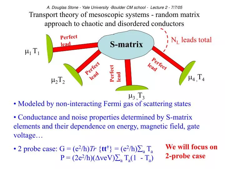
A. Douglas Stone - Yale University -Boulder CM school - Lecture 2 - 7/7/05 Transport theory of mesoscopic systems - random matrix approach to chaotic and disordered conductors Perfect lead NL leads total S-matrix 1 T1 Perfect lead Perfect lead Perfect lead 4 ,T4 2T2 3 ,T3 • Modeled by non-interacting Fermi gas of scattering states • Conductance and noise properties determined by S-matrix elements and their dependence on energy, magnetic field, gate voltage… • 2 probe case: G = (e2/h)Tr {tt†} = (e2/h)a Ta P = (2e2/h)(eV)a Ta(1 - Ta) We will focus on 2-probe case
S Disordered metal Weak localizationUCF , anomalous shot noise, anomalous thermopower… Ballistic point contact ballistic What’s in the Box? But not a result of adiabaticity! See Szafer and Stone PRL 1989
Ballistic open quantum dot • Two approaches to understanding S-matrix: • Semiclassical/statistical: dynamical/flexible (JBS 1990, 93,Marcus 1992) • Random matrix theory (hard chaos, purely statistical) (1994) (Wigner, Dyson, Mehta…1950s - 1960s - Nuclear Physics; Quantum Chaos, BGS 1984; MesoPhys: Alt-Shkl. 1986, Imry 1986, Ballistic: Mello,Bar + Jalabert,Pich,Been 1994) • Disordered Quasi-1D: Imry 1986, Muttalib et al. 1987, Dorokhov (1983) &MPK (1988), Beenakker (97) - relation to localization goes back to 1960’s • Belief: SC approach gave dynamical info, but not quantitative (see 1994 LH lectures); 2002 - Richter and Sieber solved problem!
Actual data from ballistic junction -M. Keller and D. Prober 1995 In both disordered and chaotic case it will be necessary to define ensembles and calculate averages over them - compare to exp’t? Ergodic hypothesis:(Lee and Stone, 1985)
S I =><=O O’=><=I’ RMT of Ballistic Microstructures Need P({Tn}), then can calculate <G>, Var(G), <Pshot> … {Tn} derived from S-matrix, need to define ensemble of S-matrices: ==> Most random distribution allowed by symmetry SS† = 1 (no TR), S = ST (with TR symmetry) S relates flux in to flux out, e-vectors and e-values not simply related to {Tn} e-values of MM† related to {Tn}, also M multiplicative - crucial for disordered case (later) - defined parameterization of S we need.
e.g 2D space: P(x,y)dxdy Random areaA What does “most random” mean for an ensemble of matrices? Most random : P(x,y)dxdy = dxdy/(Area)(dr) = dxdy/A Change variables: r, -> (dr) = rdrd/A Where from? dr·dr = dx2+dy2= dr2 + (rd)2 = ∑ij gijqiqj => (dr) = (det[g])1/2 Need P(S), P(M), P(H)… must define space and metric for matrices Dim. = # of ind. Parameters = 4N2, N(2N+1); N channels, 2N x 2N matrices - what is metric?dS2 = Tr{dSdS†} -> g -> (dS) = (det[g])1/2 Example: 2 x 2 real symmetric matrix (TR inv. TLS hamiltonian)
More useful coordinate system: E-values + e-vectors Eigenvalue repulsion, non-trivial metric = 1,2,4 for 3 symm. classes
Parameterize M, then S: “polar decomposition” = Diag(1, 2, …N), uiare N x N unitary matrices, with TR: u3 = u1*, u4 = u2*. Find (dM) in terms of {a}, then P({a}) => P({Ta}), avg.s of g Can work directly with S
MesoNoise WL UCF Have the j.p.d, what do we need to do with it? For Var(g) need Need 1-pt and 2-pt correlation fcns of the jpd of {Tn}
Use recursion relations, asymptotic form of pn : (normalized to N - so that G = (e2/h) T Many methods to find these fcns and the two-pt corr. fcn is “universal” upon rescaling if only logarithmic correlations Nice approach for =2 is method of orthogonal polynomials pn= orthog poly, choose Legendre, [0,1] Same method gives K(T,T’) in terms of pN pN-1
(T)/N 0 1 T What do we expect for this system? Classical symmetry betweeen reflection and transmission => <R> = <T> = N/2 Need to go to next order in N-1 to get WL effect
Coherent backscattering Off-diagonal correlations GWL = (e2/h)(1/4) Due to symmetry between reflection and transmission can get order 1/N effects easily for the circular ensemble - don’t need to distinguish Tab, Rab = Sab just do averages over unitary group U(2N) Similarly Var(g) = (1/8) The Mystery
All of these results are subtly different for a disordered/diffusive wire - will analyze next lecture