Download

1 / 37
390 likes | 693 Views
Discrete Probability Distributions. Random variables Discrete probability distributions Expected value and variance Binomial probability distribution. Random Variables. A random variable is a numerical description of the outcome of an experiment. Discrete Random Variables.

E N D
Discrete Probability Distributions • Random variables • Discrete probability distributions • Expected value and variance • Binomial probability distribution
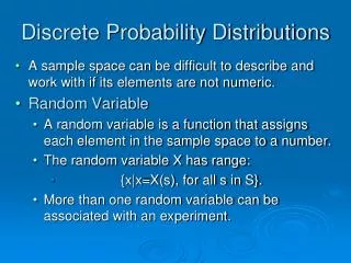
Random Variables A random variable is a numerical description of the outcome of an experiment
Discrete Random Variables A discrete random variable may assume a finite number of numerical values or an infinite sequence of values such as 0, 1, 2, . . . Example: 1 = passed driving test 2 = failed driving test This is a discrete variable because it is either pass or fail—you can’t score 1½, for example. Notice also it assumes a finite number of values
Example: JSL Appliances • Discrete random variable with an infinite sequence of values Let x = number of customers arriving in one day, where x can take on the values 0, 1, 2, . . . We can count the customers arriving, but there is no finite upper limit on the number that might arrive.
Continuous Random Variables Continuous random variables can assume an infinite number of values within a defined interval. The liquid in these bottles (x) must be between 0 and 32 ounces. But x could be 2 oz., 2.1 oz., 2.01 oz, 2.001 oz., . . .
Random Variables Type Random Variable x Question Family size x = Number of dependents in family reported on tax return Discrete x = Distance in miles from home to the store site Distance from home to store Continuous Own dog or cat Discrete x = 1 if own no pet; = 2 if own dog(s) only; = 3 if own cat(s) only; = 4 if own dog(s) and cat(s)
Discrete Probability Distributions The probability distribution is defined by a probability function, denoted by f(x), which provides the probability for each value of the random variable. The required conditions for a discrete probability function are: f(x) > 0 f(x) = 1
Using past data on TV sales, … Example: JSL Appliances • a tabular representation of the probability distribution for TV sales was developed. Number Units Soldof Days 0 80 1 50 2 40 3 10 4 20 200 xf(x) 0 .40 1 .25 2 .20 3 .05 4 .10 1.00 80/200
.50 .40 .30 .20 .10 Example: JSL Appliances • Graphical Representation of the Probability Distribution Probability 0 1 2 3 4 Values of Random Variable x (TV sales)
This is the simplest probability distribution described by a formula. It assumes that possible values of random variables are equally likely Discrete Uniform Probability Distribution n = number of values the random variable may assume.
Example: Rolling a Die Note that n = 6
Expected Value E(x) The expected value, or mean, of a random variable, is a measure of central location for the random variable For a discrete random variable x we have
Notice that this is a weighted average of the values a random variable can assume. The “weights” are the probabilities.
Example: JSL Appliances xf(x)xf(x) 0 .40 .00 1 .25 .25 2 .20 .40 3 .05 .15 4 .10 .40 E(x) = 1.20 • Expected Value of a Discrete Random Variable expected number of TVs sold in a day
Variance of a Discrete Random Variable The variance of a random variable x is a weighted average of the squared deviations of a random variable from its mean (expected) value. The weights are the probabilities.
Example: JSL Appliances x (x - )2 f(x) (x - )2f(x) x - -1.2 -0.2 0.8 1.8 2.8 1.44 0.04 0.64 3.24 7.84 0 1 2 3 4 .40 .25 .20 .05 .10 .576 .010 .128 .162 .784 • Variance and Standard Deviation of a Discrete Random Variable TVs squared Variance of daily sales = s 2 = 1.660 Standard deviation of daily sales = 1.2884 TVs
Using Excel to Compute the Expected Value, Variance, and Standard Deviation • Formula Worksheet
Using Excel to Compute the Expected Value, Variance, and Standard Deviation • Value Worksheet
The Binomial Distribution This is a very useful tool for multi-step experiments where each step has 2 outcomes—hence the term binomial.
Properties of Binomial Experiment • The experiment consists of a sequence of n identical trials. • Two outcomes are possible on each trial. We refer to one outcome as a success and the other outcome as a failure. • The probability of success, denoted by ρ, does not change from trial to trial. Consequently, the probability of failure, denoted by 1 – ρ , does not change from trial to trial. • The trials are independent. Stationarity assumption
We are interested in computing the number of successes (x) for n number of trials
Binomial Probability Distribution The binomial distribution is given by: Where: f(x) = probability of success in n trials n = number of trials p = probability of success in any one trial.
Example: Evans Electronics • Binomial Probability Distribution Evans is concerned about a low retention rate for employees. In recent years, management has seen a turnover of 10% of the hourly employees annually. Thus, for any hourly employee chosen at random, management estimates a probability of 0.1 that the person will not be with the company next year.
If we selected three (3) employees at random, what is the probability that one(1) will leave the company within the year? Evans electronics • Notice that: • The experiment has three identical trials—that is, n = 3. • There are two outcomes for each trial—the employee leaves (S) or the employee stays (F). • The probability that an employee will leave is .1—that is, ρ = .1 • The decision of each employee to leave is independent of the decisions made by the other employees.
FirstEmployee SecondEmployee ThirdEmployee ExperimentalOutcome Value of x32212110 Counting the Number of Outcomes (S,S,S) S S F (S,S,F) F S (S,F,S) S F (S,F,F) S F S (F,S,S) (F,S,F) F F S (F,F,S) (F,F,F) F
Number of Experimental Outcomes Providing Exactly x Successes in n trials In our Evans Electronics example, n = 3 and x = 1. Thus: Refer to the tree diagram to verify this is right
What is the probability the first employee selected will leave and second and third will stay? Note this is outcome (S, F, F) Because these events are independent, we can multiply probabilities. . Thus the probability of (S, S, F) is given by: Thus we have:
Binomial Probability Distribution • Binomial Probability Function Probability of a particular sequence of trial outcomes with x successes in n trials Number of experimental outcomes providing exactly x successes in n trials
Probability Distribution for the Number of Employees Leaving Within the Year
Using Excel to ComputeBinomial Probabilities • Formula Worksheet
Using Excel to ComputeBinomial Probabilities • Value Worksheet
Using Excel to ComputeCumulative Binomial Probabilities • Formula Worksheet
Using Excel to ComputeCumulative Binomial Probabilities • Value Worksheet
Expected Value and Variance for a Binominal Distribution The expected value is computed by: The variance is computed by:
Evans Electronics Example Remember that n = 3 and ρ = .1. Thus: Note also that: