Download
1 / 46
470 likes | 756 Views
Equilibrium, Shear Stress, Stream Power and Trends of Vertical Adjustment. Andrew Simon USDA-ARS National Sedimentation Laboratory, Oxford, MS andrew.simon@ars.usda.gov. Non-Cohesive versus Cohesive Materials. Non-cohesive: sands and gravels etc.

E N D
Equilibrium, Shear Stress, Stream Power and Trends of Vertical Adjustment Andrew Simon USDA-ARS National Sedimentation Laboratory, Oxford, MS andrew.simon@ars.usda.gov
Non-Cohesive versus Cohesive Materials • Non-cohesive: sands and gravels etc. • Resistance is due solely to particle size, weight, shape and “hiding”. • Cohesive: silts and clays • Resistance is derived from electro-chemical inter-particle forces under zero normal stress
Shields Diagram Cohesive Materials Denotes uncertainty
Shields Diagram by Particle Diameter Excludes cohesives
Heterogeneous Beds ks = 3* D84
Erosion of Cohesives by Hydraulic Shear National Sedimentation Laboratory Need for a means to determine critical shear stress (tc) and the erodibility coefficient (k) in-situ for soils and sediments.
Erosion Rate is a Function of Erodibility and Excess Shear Stress e = k (to- tc) e = erosion rate (m/s) k = erodibility coefficient (m3/N-s) to =boundary shear stress (Pa) tc =critical shear stress (Pa) (to-tc) = excess shear stress Critical shear stress is the stress required to initiate erosion. Obtained from jet-test device
Impinging Jet Applies Shear Stress to Bed National Sedimentation Laboratory Jet Nozzle
Impinging Jet Applies Shear Stress to Bed National Sedimentation Laboratory Jet Nozzle As scour hole depth increases, shear stress decreases.
From Relation between Shear Stress and Erosion We Calculate tc and e National Sedimentation Laboratory tc Erosion Depth, cm (cm3/Pa/sec) k Time
General Relation for Erodibility and Critical Shear Stress Erodibility, m3/N-s k = 0.1 tc -0.5 Where; tc = critical shear stress (Pa), x, y = empirical constants
Mapping Critical Shear Stress: Yalobusha River Basin, Mississippi National Sedimentation Laboratory
Idealized Adjustment TrendsFor a given discharge (Q) National Sedimentation Laboratory t gVS Se n tc d
Boundary Shear Stress: Range of Flows Shearstress, in N/m2
Adjustment: Excess Shear StressDegrading Reach Excess shear stress
Results of AdjustmentDecreasing Sediment Loads with Time Toutle River System
Total and Unit Stream Power • W = g w y V S = g Q S • W = total stream power per unit length of channel • g = specific weight of water • w = water-surface width • y = hydraulic depth • v = mean flow velocity • Q = water discharge • S = energy slope • ww = W / (g w y) = V S • where ww = stream power per unit weight of water
Flow Energy • Total Mechanical Energy H = z + y + (a v2/ 2 g) where H = total mechanical energy (head) z = mean channel-bed elevation (datum head) a = coefficient for non-uniform distribution velocity y = hydraulic depth (pressure head) g = acceleration of gravity • Head Loss over a reach due to Friction hf = [z1 + y1 + (a1 v12/ 2g)]- [z2 + y2 + (a2 v22/ 2g)] • Head, Relative to channel bed Es = y + (av2/ 2g) =y + [a Q2 / (2 g w2 y2)]
Adjustment: Total Mechanical Energy As a working hypothesis we assume that a fluvial system has been disturbed in a manner such that the energy available to the system (potential and kinetic) has been increased. We further assume that with time, the system will adjust such that the energy at a point (head) and the energy dissipated over a reach (head loss), is decreased. Now, for a given discharge, consider how different fluvial processes will change (increase or decrease) the different variables in the energy equations.
Adjustment: Energy Dissipation Minimization of energy dissipation
Determining Equilibrium Recall definition A stream in equilibrium is one in which over a period of years, slope is adjusted such that there is no net aggradation or degradation on the channel bed (or widening or narrowing) OR There is a balance between energy conditions at the reach in question with energy and materials being delivered from upstream
Empirical Functions to Describe Incision E = a t b E = elevation of the channel bed a = coefficient; approximately, the pre-disturbance elevation t = time (years), since year before start of adjustment b = dimensionless exponent indicating rate of change on the bed (+) for aggradation, (-) for degradation E/ Eo = a +b e-kt E = elevation of the channel bed Eo = initial elevation of the channel bed a = dimensionless coefficient, = the dimensionless elevation a > 1 = aggradation, a < 1 = degradation b = dimensionless coefficient, = total change of elevation b > 0 = degradation, b < 0 = aggradation k = coefficient indicating decreasing rate of change on the bed
Bed Response: Toutle River System Upstream disturbance, addition of potential energy, sub-alpine environment
Comparison with Coastal Plain Adjustment Downstream disturbance, increase in gradient, coastal plain environment