Download
1 / 29
290 likes | 377 Views
What Do We Know About MHD Turbulence?. IAEA Technical Workshop Trieste 2005. The Equations:. and.

E N D
What Do We Know About MHD Turbulence? IAEA Technical Workshop Trieste 2005
TheEquations: and These are toy equations, in the sense that viscosity and resistivity are included in the simplest possible way, and as constants. In dense environments (inside stars and accretion disks) this can be ~realistic, but in general it’s not. Compressibility is also neglected, although I will relax this assumption later.
Outline: • Theory --- the early years • Observations --- the solar wind and the ISM • Goldreich-Sridhar model for strong turbulence • Numerical Simulations - power spectra, intermittency, pdf, transport • Miscellaneous - physics of the energy cascade, compressibility • Summary
Modes in Incompressible MHD 1. Alfven waves: 2. Pseudo-Alfven waves (slow modes): Both modes propagate along field lines at VA
Alfvenic Turbulence: The Iroshnikov-Kraichnan Model (I63, K65) Assume an ensemble of waves, distributed isotropically in phase space and interacting weakly. The nonlinear interaction rate is reduced by the ratio of the advective rate to the wave frequency, or Then Since v decreases as k increases, the waves become increasingly weakly interacting.
Isotropy? Since the large scale magnetic field appears in the dynamical equations in the combination we can compare this to the advective rate We see that we can define two classes of modes, depending on which rate is higher, (Alfven waves and zero-frequency vortices) and these modes will have fundamentally different dynamical properties. The assumption of isotropy is not self-consistent. These classes are usually called “slab turbulence” and “2D turbulence”.
“Reduced MHD” (Rosenbluth, Strauss) assumes that the magnetic field is stiff, so that This ratio is also assumed to describe the ratio of b to B0 while slow modes are dropped. MHD turbulence is often modeled as a superposition of “slab” and “2D” modes. The boundary between them was not initially assumed to have much weight. Early simulations aimed at studying mode anisotropy (e.g. Shebalin et al. 1983) seemed to show that the degree of anisotropy in a turbulent cascade is set at the largest scales, so that is a constant. This validates the IK scaling giving a 1D spectral index of -3/2 for the cascade.
Turbulence in the Solar Wind From Leamon et al. 1998 - Typical power spectrum for stationary states of the solar wind. The cascade extends from ~10-4 Hz to a fraction of Hz.
Armstrong & Spangler (1995) Slope ~ -5/3 Electron density spectrum pc AU
The Goldreich-Sridhar Model (1995) Resonant 3-wave interactions vanish for Alfven waves. GS showed the 4-wave interactions could produce strong turbulence with the following properties: • The advective and Alfven rates are comparable at every level in the turbulent cascade. • Alfven waves have coherence times comparable to the inverse of these rates, that is, about one wave period. • The cascade shows a scale-dependent level of anisotropy. Smaller eddies are more elongated along the field direction. They also concluded that all higher order interactions contributed corrections of order unity.
That turns out not be as bad as it sounds (or I wouldn’t cite their work at all). 2D turbulence has an inverse energy casdade. The perpendicular wavenumber will decrease (and the parallel wavenumber increase via a random walk) so the eddies work back towards the limit where the Alfven frequency is significant. On the other hand, 4-wave interactions among Alfven waves will increase the perpendicular wavenumber, while the parallel wavenumber stays constant. So left to themselves, either slab modes or 2D modes will evolve towards the balance where
The Energy Spectrum Since there is only one rate, the turbulent cascade looks just like the Kolmogorov cascade, except that we only deal in perpendicular velocities and wavenumbers. On the other hand, the rate balance condition gives Smaller eddies are more elongated.
Where are pseudo-Alfven modes in all of this? To leading order, PA modes do not transfer power to high wavenumbers via nonlinear interactions with other PA modes. They do this via interactions with Alfven waves. They have no effect on Alfven waves. The prediction is that the power spectrum of PA modes should look much like that of the Alfven modes, but if some mechanism suppresses these modes, there will be no effect on the Alfven modes or their turbulent cascade. This is important because in collisionless systems, PA modes are strongly damped through parallel transport.
|B| B0 The theoretical and observational developments of the ‘90s were parallel by technological improvements that made it possible to perform detailed 3D MHD simulations. From Cho & Vishniac (2000) See also Muller & Biskamp (2000); Maron & Goldreich (2001)
Does this settle the issue? No The simulations by Maron and Goldreich, and more recent simulations by Muller and Biskamp, seem to argue for the IK power spectrum. I think this is an unresolved issue, and raises observational difficulties. The other prediction in GS is that eddies should show a scale dependent elongation. This can also be checked in simulations, but first we need to address why this effect was not seen by Shebalin et al.
Averaging over a turbulent system using a global definition of the magnetic field direction will smear out small scale anisotropies, leaving only those due to the largest scale eddies. This is what Shebalin et al. saw.
Anisotropy in the Numerical Simulations Contours in the velocity structure function (Cho and Vishniac). Similar results in MG, MB, and Milano et al. The shape of the contours closely match the GS model. Plots of magnetic field structure functions are very similar.
What is the PDF for Magnetic Fluctuations? From the simulations, the correlation tensor for the magnetic field scales as for a given value of and large values of This is consistent with observations of the solar wind, although in this case the data is sufficient to argue that a more complete description is given by a Castaing distribution (Forman and Burlaga).
Intermittency in Turbulence: Structure Function Exponents MHD turbulence is anisotropic, so we need to specify if we are looking at correlation along the field lines or across them. We also need to specify whether directions are defined relative to the local magnetic field, or a global magnetic field direction. The scaling exponents are connected to the details of the energy cascade (among other things).
She-Leveque Model of intermittency C is the codimension of the dissipative structures, e.g. vortices in hydrodynamic turbulence imply C=2. For example, for p=2 we get =0.696 (as opposed to 2/3). If we assumed instead that hydrodynamic turbulence forms dissipatative sheets we would get =0.741. The effect of C gets larger as p increases.
Suppose we look along the local field direction, that is, take The errors in (p) become much larger, since it is hard to track the magnetic field lines with the required accuracy. For the velocity field, the results are consistent with multiplying the previously derived set of exponents by 3/2. The velocity structure of the turbulence is simply stretched by a scale dependent factor which follows the proposed Goldreich-Sridhar scaling.
What Have We Learned From (p)? • The velocity and magnetic fields behave as though they are controlled by dissipation structures with different dimensions, despite the transfer of energy between them. • The velocity field looks very much like hydrodynamic turbulence, stretched along the local field direction. • Elsasser variables can be misleading in the limit of strong turbulence.
The Physics of the MHD Turbulent Cascade --- as if I knew Reading off the Elsasser variable intermittency exponents suggests a simple picture with 2D dissipative structures. Looking at the velocity and magnetic field results separately seems to suggest that there are two sets of dissipative structures: vortices (1D), and current sheets (2D). Moreover, looking at the results in the local frame suggests that the effective dimension of the magnetic structures is slightly greater than 2. Perhaps a fractal distribution of current sheets, with partially aligned vortex tubes?
Compressible Turbulence Adding compressibility opens up the possibility of fast magnetosonic waves. If we go to the supersonic, but sub-Alfvenic, limit, we see very little change in the properties of the Alfven waves and the slow modes. However, the fast waves look dramatically different.
We get isotropic sonic turbulence with a spectral index of 3/2. The fast waves follow the model proposed by Iroshnikov and Kraichnan. Despite collisionless damping in the ISM, these waves dominate the scattering of cosmic rays by about 15 orders of magnitude. (Yan and Lazarian)
Summary • There exists a theory for MHD turbulence, roughly comparable to the original work of Kolmogorov, describing the strong turbulent MHD cascade. It is the model proposed in GS95. It is also equivalent to assuming that “typical” modes satisfy the ordering given in reduced MHD. This model successfully predicts eddy shapes • However, the power spectrum of incompressible MHD turbulence is still uncertain. This may be explained by intermittency.
More Summary: • If we look directly at intermittency statistics, we see that the velocity field is like hydrodynamic turbulence, stretched along the magnetic field lines. On the other hand, the magnetic field is strikingly more intermittent. This hints at significantly different roles in the energy cascade. • The PDF of the simulations matches that in the solar wind. It is not predicted from first principles.