Uptake, Storage, and Transport:

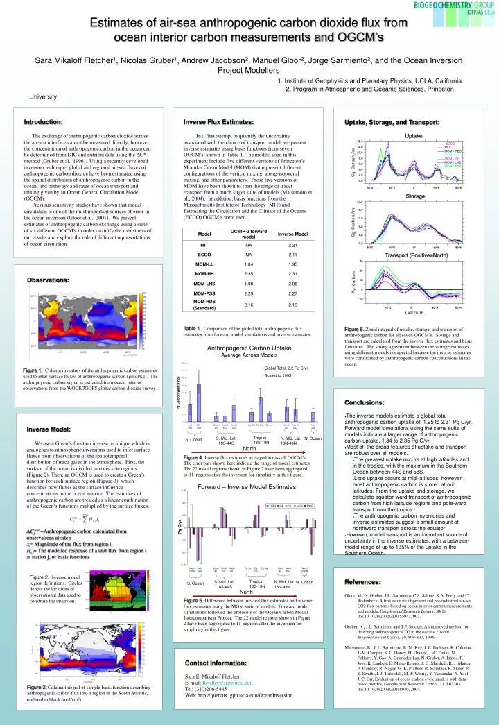
1. Forward – Inverse Model Estimates Tropics 18S-18N S. Mid. Lat. 18S-44S N. Mid. Lat. 18N-49N N. Ocean S. Ocean Tropics 18S-18N S. Mid. Lat. 18S-44S N. Mid. Lat. 18N-49N N. Ocean S. Ocean North North Anthropogenic Carbon UptakeAverage Across Models Global Total: 2.2 Pg C/yr Scaled to 1995 Estimates of air-sea anthropogenic carbon dioxide flux from ocean interior carbon measurements and OGCM’s Sara Mikaloff Fletcher1, Nicolas Gruber1, Andrew Jacobson2, Manuel Gloor2, Jorge Sarmiento2, and the Ocean Inversion Project Modellers 1. Institute of Geophysics and Planetary Physics, UCLA, California 2. Program in Atmospheric and Oceanic Sciences, Princeton University Introduction: The exchange of anthropogenic carbon dioxide across the air-sea interface cannot be measured directly; however, the concentration of anthropogenic carbon in the ocean can be determined from DIC and nutrient data using the ∆C* method (Gruber et al., 1996). Using a recently developed inversion technique, global and regional air-sea fluxes of anthropogenic carbon dioxide have been estimated using the spatial distribution of anthropogenic carbon in the ocean, and pathways and rates of ocean transport and mixing given by an Ocean General Circulation Model (OGCM). Previous sensitivity studies have shown that model circulation is one of the most important sources of error in the ocean inversion (Gloor et al., 2001). We present estimates of anthropogenic carbon exchange using a suite of six different OGCM's in order quantify the robustness of our results and explore the role of different representations of ocean circulation. Inverse Flux Estimates: In a first attempt to quantify the uncertainty associated with the choice of transport model, we present inverse estimates using basis functions from seven OGCM’s, shown in Table 1. The models used in this experiment include five different versions of Princeton’s Modular Ocean Model (MOM) that represent different configurations of the vertical mixing, along-isopycnal mixing, and other parameters. These five versions of MOM have been shown to span the range of tracer transport from a much larger suite of models (Matsumoto et al., 2004). In addition, basis functions from the Massachusetts Institute of Technology (MIT) and Estimating the Circulation and the Climate of the Oceans (ECCO) OGCM’s were used. Table 1.Comparison of the global total anthropogenic flux estimates from forward model simulations and inverse estimates. Figure 4.Inverse flux estimates averaged across all OGCM’s. The error bars shown here indicate the range of model estimates. The 22 model regions shown in Figure 2 have been aggregated to 11 regions after the inversion for simplicity in this figure. Figure 5.Difference between forward flux estimates and inverse flux estimates using the MOM suite of models. Forward model simulations followed the protocols of the Ocean Carbon Model Intercomparison Project. The 22 model regions shown in Figure 2 have been aggregated to 11 regions after the inversion for simplicity in this figure. Uptake, Storage, and Transport: Figure 6.Zonal integral of uptake, storage, and transport of anthropogenic carbon for all seven OGCM’s. Storage and transport are calculated from the inverse flux estimates and basis functions. The strong agreement between the storage estimates using different models is expected because the inverse estimates were constrained by anthropogenic carbon concentrations in the ocean. Uptake - - - - ECCO - - - - MIT —— MOM - RDS —— MOM - LL —— MOM - HH —— MOM - LHS —— MOM - PSS Storage Transport (Positive=North) Observations: Figure 1.Column inventory of the anthropogenic carbon estimates used to infer surface fluxes of anthropogenic carbon (μmol/kg). The anthropogenic carbon signal is extracted from ocean interior observations from the WOCE/JGOFS global carbon dioxide survey. Conclusions: • The inverse models estimate a global total anthropogenic carbon uptake of 1.95 to 2.31 Pg C/yr. Forward model simulations using the same suite of models indicate a larger range of anthropogenic carbon uptake, 1.84 to 2.35 Pg C/yr. • Most of the broad features of uptake and transport are robust over all models. • The greatest uptake occurs at high latitudes and in the tropics, with the maximum in the Southern Ocean between 44S and 58S. • Little uptake occurs at mid-latitudes; however, most anthropogenic carbon is stored at mid latitudes. From the uptake and storage, we calculate equator-ward transport of anthropogenic carbon from high latitude regions and pole-ward transport from the tropics. • The anthropogenic carbon inventories and inverse estimates suggest a small amount of northward transport across the equator • However, model transport is an important source of uncertainty in the inverse estimates, with a between-model range of up to 135% of the uptake in the Southern Ocean. Inverse Model: We use a Green’s function inverse technique which is analogous to atmospheric inversions used to infer surface fluxes from observations of the spatiotemporal distribution of trace gases in the atmosphere. First, the surface of the ocean is divided into discrete regions (Figure 2). Then, an OGCM is used to create a Green’s function for each surface region (Figure 3), which describes how fluxes at the surface influence concentrations in the ocean interior. The estimates of anthropogenic carbon are treated as a linear combination of the Green’s functions multiplied by the surface fluxes. ∆Cjant=Anthropogenic carbon calculated from observations at site j xi= Magnitude of the flux from region i Hi,j= The modelled response of a unit flux from region i at station j, or basis functions References: Gloor, M., N. Gruber, J.L. Sarmiento, C.S. Sabine, R.A. Feely, and C. Rödenbeck, A first estimate of present and pre-industrial air-sea CO2 flux patterns based on ocean interior carbon measurements and models, Geophysical Research Letters, 30(1), doi:10.1029/2002GL015594, 2003. Gruber, N., J.L. Sarmiento and T.F. Stocker, An improved method for detecting anthropogenic CO2 in the oceans. Global Biogeochemical Cycles, 10, 809-837, 1996. Matsumoto, K., J. L. Sarmiento, R. M. Key, J. L. Bullister, K. Caldeira, J.-M. Campin, S. C. Doney, H. Drange, J.-C. Dutay, M. Follows, Y. Gao, A. Gnanadesikan, N. Gruber, A. Ishida, F. Joos, K. Lindsay, E. Maier-Reimer, J. C. Marshall, R. J. Matear, P. Monfray, R. Najjar, G.-K. Plattner, R. Schlitzer, R. Slater, P. S. Swathi, I. J. Totterdell, M.-F. Weirig, Y. Yamanaka, A. Yool, J. C. Orr, Evaluation of ocean carbon cycle models with data- based metrics, Geophysical Research Letters, 31, L07303, doi:10.1029/2003GL018970, 2004. Figure 2.Inverse model region definitions. Circles denote the locations of observational data used to constrain the inversion. Contact Information: Sara E. Mikaloff Fletcher E-mail: fletcher@igpp.ucla.edu Tel: (310)206-5445 Web: http://quercus.igpp.ucla.edu/OceanInversion Figure 3: Column integral of sample basis function describing anthropogenic carbon flux into a region in the South Atlantic, outlined in black (mol/cm2).