Download
1 / 28
300 likes | 486 Views
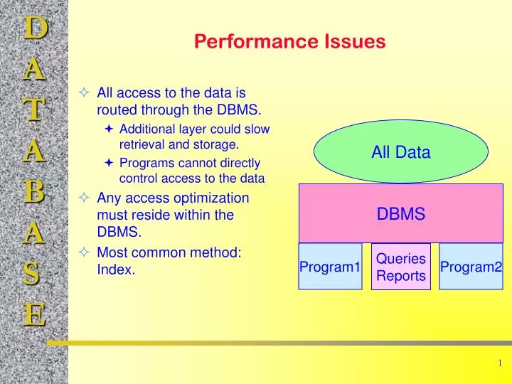
All access to the data is routed through the DBMS. Additional layer could slow retrieval and storage. Programs cannot directly control access to the data Any access optimization must reside within the DBMS. Most common method: Index. Performance Issues. All Data. DBMS. Program1. Program2.

E N D
All access to the data is routed through the DBMS. Additional layer could slow retrieval and storage. Programs cannot directly control access to the data Any access optimization must reside within the DBMS. Most common method: Index. Performance Issues All Data DBMS Program1 Program2 Queries Reports
Some database systems let the designer choose how to store data. Rows for each table. Columns within a table. The choice influences performance and storage requirements. The choice depends on the characteristics of the data being stored. Index Most database systems use an index to improve performance. Several methods can be used to store an index. An index can speed data retrieval. Maintaining many indexes on a table can significantly slow down data updates and additions. Choose indexes carefully to speed up certain large jobs. Physical Data Storage
Retrieve data Read entire table. Read next row/sequential. Read arbitrary/random row. Store data Insert a row. Delete a row. Modify a row. Reorganize/pack database Remove deleted rows. Recover unused space. Table Operations LastName FirstName Phone Adams Kimberly (406) 987-9338 Adkins Inga (706) 977-4337 Allbright Searoba (619) 281-2485 Anderson Charlotte (701) 384-5623 Baez Bessie (606) 661-2765 Baez Lou Ann (502) 029-3909 Bailey Gayle (360) 649-9754 Bell Luther (717) 244-3484 Carter Phillip (219) 263-2040 Cartwright Glen (502) 595-1052 Carver Bernice (804) 020-5842 Craig Melinda (502) 691-7565
Deletes are flagged. Space is reused if possible when new row is added. If not exactly the same size, some blank holes develop. Packing removes all deleted data and removes blanks. Deleting Data LastName FirstName Phone Adams Kimberly (406) 987-9338 Adkins Inga (706) 977-4337 Allbright Searoba (619) 281-2485 Anderson Charlotte (701) 384-5623 Baez Bessie (606) 661-2765 XBaez Lou Ann (502) 029-3909 Bailey Gayle (360) 649-9754 Bell Luther (717) 244-3484 Carter Phillip (219) 263-2040 Cartwright Glen (502) 595-1052 Carver Bernice (804) 020-5842 Craig Melinda (502) 691-7565
Data Storage Methods • Sequential • Fast for reading entire table. • Slow for random search. • Indexed Sequential (ISAM) • Better for searches. • Slow to build indexes. • B+-Tree • Similar to ISAM. • Efficient at building indexes. • Direct / Hashed • Extremely fast searches. • Slow sequential lists.
Common uses When large portions of the data are always used at one time. e.g., 25% When table is huge and space is expensive. When transporting / converting data to a different system. Sequential Storage
Read entire table Easy and fast Sequential retrieval Easy and fast for one order. Random Read/Sequential Very weak Probability of any row = 1/N Sequential retrieval 1,000,000 rows means 500,000 retrievals per lookup! Delete Easy Insert/Modify Very weak Operations on Sequential Tables Row Prob. # Reads A 1/N 1 B 1/N 2 C 1/N 3 D 1/N 4 E 1/N 5 … 1/N i
Insert Inez: Find insert location. Copy top to new file. At insert location, add row. Copy rest of file. Insert into Sequential Table
When data is stored on drive (or RAM). Operating System allocates space with a function call. Provides location/address. Physical address Virtual address (VSAM) Imaginary drive values mapped to physical locations. Relative address Distance from start of file. Other reference point. Pointers Address Data • Volume • Track • Cylinder/Sector • Byte Offset • Drive Head Key value Address / pointer
Common uses Large tables. Need many sequential lists. Some random search--with one or two key columns. Mostly replaced by B+-Tree. Indexed Sequential Storage Address ID LastName FirstName DateHired 1 Reeves Keith 1/29/2001 2 Gibson Bill 3/31/2001 3 Reasoner Katy 2/17/2001 4 Hopkins Alan 2/8/ 2001 5 James Leisha 1/6/ 2001 6 Eaton Anissa 8/23/ 2001 7 Farris Dustin 3/28/ 2001 8 Carpenter Carlos 12/29/ 2001 9 O'Connor Jessica 7/23/ 2001 10 Shields Howard 7/13/ 2001 A11 A22 A32 A42 A47 A58 A63 A67 A78 A83 ID Pointer 1 A11 2 A22 3 A32 4 A42 5 A47 6 A58 7 A63 8 A67 9 A78 10 A83 LastName Pointer Carpenter A67 Eaton A58 Farris A63 Gibson A22 Hopkins A42 James A47 O'Connor A78 Reasoner A32 Reeves A11 Shields A83 Indexed for ID and LastName
Given a sorted list of names. How do you find Jones. Sequential search Jones = 10 lookups Average = 15/2 = 7.5 lookups Min = 1, Max = 14 Binary search Find midpoint (14 / 2) = 7 Jones > Goetz Jones < Kalida Jones > Inez Jones = Jones (4 lookups) Max = log2 (N) N = 1000 Max = 10 N = 1,000,000 Max = 20 Binary Search Adams Brown Cadiz Dorfmann Eaton Farris 1 Goetz Hanson 3 Inez 4 Jones 2 Kalida Lomax Miranda Norman 14 entries
Separate each element/key. Pointers to next element. Pointers to data. Starting point. A67 8 Carpenter Carlos 12/29/2001 A22 2 Gibson Bill 3/31/2001 B29 Eaton B71 A58 B87 Carpenter B29 A67 B38 Gibson 00 A22 A58 6 Eaton Anissa 8/23/2001 A63 7 Farris Dustin 3/28/2001 B71 Farris B38 A63 Linked List
Get space/location with address. Data: Save row (A97). Key: Save key and pointer to data (B14). Find insert location. Eccles would be after Eaton and before Farris. From prior key (Eaton), put next address (B71) into new key, next pointer. Put new address (B14) in prior key, next pointer. B29 Eaton B71 A58 B71 Farris B38 A63 Insert into a Linked List B14 B14 Eccles B71 A97 NewData = new (. . .) NewKey = new (. . .) NewKey->Key = “Eccles” NewKey->Data = NewData FindInsertPoint(List, PriorKey, NewKey) NewKey->Next = PriorKey->Next PriorKey->Next = NewKey
Store key values Utilize binary search (or better). Trees Nodes Root Leaf (node with no children) Levels / depth Degree (maximum number of children per node) B-Tree < Key Data >= Hanson Dorfmann Kalida Brown Farriis Inez Miranda Adams Cadiz Eaton Goetz Jones Lomax Norman Inez A B C D E F G H I J K L M N
Special characteristics Set the degree (m) m >= 3 Usually an odd number. Every node (except the root) must have between m/2 and m children. All leaves are at the same level/depth. All key values are displayed on the bottom leaves. A nonleaf node with n children will contain n-1 key values. Leaves are connected by pointers (sequential access). Example data 156, 231, 287, 315 347, 458, 692, 792 B+-Tree
Degree 3 At least m/2 = 1.5 (=2) children. No more than 3 children. Search keys (e.g., find 692) Less than Between Greater than Sequential links. B+-Tree Example < 315 <= < 231 <= < 287 <= < 458 <= < 792 <= < 156 <= < 231 <= < 287 <= < 315 <= < 347 <= < 458 <= < 692 <= < 792 <= data
Insert 257 Find location. Easy with extra space. Just add element. B+-Tree Insert < 315 <= < 231 <= < 287 <= < 458 <= < 792 <= < 156 <= < 287 <= < 315 <= < 347 <= < 458 <= < 692 <= < 792 <= < 231 <= < 257 <=
Insert 532 Find location. Cell is full. Move up a level, cell is full. Move up to top and split. Eventually, add a level. B+-Tree Insert < 315 <= < 231 <= < 287 <= < 458 <= < 792 <= < 156 <= < 231 <= < 257 <= < 287 <= < 315 <= < 347 <= < 458 <= < 692 <= < 792 <= < 315 <= < 692 <= < 231 <= < 287 <= < 347 <= < 458 <= < 692 <= < 792 <= < 156 <= < 231 <= < 287 <= < 315 <= < 347 <= < 458 <= < 532 <= < 692 <= < 792 <=
Designed to give good performance for any type of data and usage. Lookup speed is based on degree/depth. Maximum is logm n. Sequential usage is fast. Insert, delete, modify are reasonable. Many changes are easy. Occasionally have to reorganize large sections. B+-Tree Strengths
Convert key value directly to location (relative or absolute). Use prime modulus Choose prime number greater than expected database size (n). Divide and use remainder. Set aside spaces (fixed-length) to hold each row. Collision/overflow space for duplicates. Extremely fast retrieval. Very poor sequential access. Reorganize if out of space! Example Prime = 101 Key = 528 Modulus = 23 Direct Access / Hashed Overflow/collisions
Choice depends on data usage. How often do data change? What percent of the data is used at one time? How big are the tables? How many joins are there? How many transactions are processed per second? Rules B+-Tree is best all-around. B+-Tree is better than ISAM Hashed is good for high-speed with random access. Sequential is good if often use entire table. Comparison of Access Methods
Different methods of storing data within each row. Positional/Fixed Simple/common. Fixed with overflow Memo/highly variable text. Storing Data Columns A101: -Extra Large A321: an-Premium A532: r-Cat
Different methods of storing data within each row. Indexed Fast access to columns. Delimited File transfer. Storing Data Columns
Clustering Grouping related data together to improve performance. Close to each other on one disk. Preferably within the same disk page or cylinder. Minimize disk reads and seeks. e.g. cluster each invoice with the matching order. Partitioning Splitting tables so that infrequently used data can be placed on slower drives. Vertical partition Move some columns. e.g., move description and comments to optical drive. Horizontal partition Move some rows. e.g., move orders beyond 2 years old to optical drive. Data Clustering and Partitioning
Keeping data on same drive Keeping data close together Same cylinder Same I/O page Consecutive sectors Data Clustering Order Order #1123 Odate C# 8876 Order# 1123 Item #078 Quantity 3 Order# 1123 Item #987 Quantity 1 Order Order #1124 Odate C# 4293 Order# 1123 Item #240 Quantity 2
Split table Horizontally Vertically Characteristics Infrequent access Large size Move to slower / cheaper storage Data Partitioning High speed hard disk Low cost optical disk Active customers Customer# Name Address Phone 2234 Inouye 9978 Kahlea Dr. 555-555-2222 5532 Jones 887 Elm St. 666-777-3333 0087 Hardaway 112 West 2000 888-222-1111 0109 Pippen 873 Lake Shore 333-111-2235
In one table, some columns are large and do not need to be accessed as often. Store primary data on high speed disk. Store other data on optical disk. DBMS retrieves both automatically as needed. Products table example. Basic inventory data. Detailed technical specifications and images. Vertical Partition High speed hard disk Low cost optical disk Item# Name QOH Description TechnicalSpecifications 875 Bolt 268 1/4” x 10 Hardened, meets standards ... 937 Injector 104 Fuel injector Designed 1995, specs . . .
Redundant Array of Independent Drives (RAID) Instead of one massive drive, use many smaller drives. Split table to store parts on different drives (striping). Duplicate pieces on different drive for backup. Drives can simultaneously retrieve portions of the data. Disk Striping and RAID CustID Name Phone 115 Jones 555-555-1111 225 Inez 666-666-2222 333 Shigeta 777-777-1357 938 Smith 888-888-2225