Download
1 / 17
180 likes | 282 Views
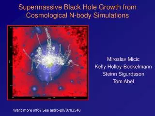
Initial conditions for N-body simulations. Hans A. Winther ITA, University of Oslo. Overview. Initial Conditions. The N-body simulation. Dynamical equations Numerical methods. A nalysis of the results Identify halos etc. Connect the simulation with observations…. Introduction.

E N D
Initial conditionsfor N-body simulations Hans A. Winther ITA, University of Oslo
Overview Initial Conditions The N-body simulation • Dynamical equations • Numerical methods • Analysis of the results • Identify halos etc. Connect the simulation with observations…
Introduction • Observations(CMB / LSS) suggests thatperturbationsstartedfrom a randomGaussianfield(completlydescribed by P(k)) put up byinflation. • Afterinflation, theevolutionoftheperturbationsarewelldescribedby • linear perturbationtheory. • Linear perturbationstheorybreaksdownwhenthedensitycontrastgets • largerthanone: N-body simulations is needed to followthe late time • smallscaleclusteringofmatter. • We are going to look at some ways to generate initial conditions in order to • perform N-body simulations
Initial conditions • N-body simulations usually starts with fairly homogenous IC. • There are different ways to place particles in the simulation box before we start the simulation. The main requirement is that the distribution is uniform. • The most obvious is to put particles on a cubic grid. • We can place particles in lattice cells, but at a random displacement from the centre of the cell. Can give large fluctuations which can lead to spurious clustering. • Place particles randomly and then evolve the distribution with repulsive gravity (glass initial conditions).
Linear perturbation theory • Remember the equations governing the evolution of the density contrast and the velocity field:
Linear perturbation theory • In the linear theory the density contrast and the velocity field is given in terms of the gravitational potential. • The problem of initial conditions reduces to generate the gravitational potential and using this to calculate the density contrast and the velocity field. • In LCDM, the linear density contrast can be written: d = c1 a + c2 a-2/3. • The Poisson equation can be written: • din = ainD2Yin and (dd/da)in= -Dvin • Which leads to • d(a) = (1/5)(3D2Yin-2Dvin)a + (2/5)(D2Yin-Dvin)a-2/3 • For a system in the growing mode we see that vin=–DYin.
Linear perturbation theory • We can now generate the initial density field in two different ways: Distribute particles uniformly and have the masses of the particles by proportional to the local density. The velocity is given by the gradient of the potential. Drawback: We have to carry an array with information about the different masses around. Distribute particles uniformly and then displace using the velocity for the growing mode. Max displacements should be smaller than the average displacement. Large displacements can lead to an incorrect realization of P(k). If this happens, recompute the gravitational potential and assign velocities again. This method can be shown to reproduce the initial density field given that the initial distribution did not have any inhomogeneities.
Zel’dovich approximation • The most widely used method to set up a quasi-linear initial condition for the N-body simulation. • Zel’dovich approximation is the first order Lagrangian perturbation theory. Normally breaks down later than Eulerian linear theory (the usual perturbation theory). • First proposed in the 1970 paper ‘Gravitational Instability: An approximate theory for large density perturbations’. Zel’dovich originally used this method to show that the first structures to form are sheets called Zel’dovich pancakes. • Assumptions: Scales of interest are smaller than the size of the horizon. The universe is dominated by dust (pressure less matter).
Zel’dovich approximation Start with some particles. The comoving position of this particle as a function of its Lagrangian position (initial position) can be written: Take the derivatives with respect to time and use perturbation theory yields:
In practice • From a power-spectrum P(k) we can make a random realization of the density field: • Where Rk=Gauss(0,1). The potential is given by: • Particles are displaced by using:
Other initial conditions • In choosing the initial conditions we also have to choose the size of the box, the number of particles and the start time. These values are not arbitrary: • We have to make sure the largest modes are in the linear regime. Starting to late can also introduce shell-crossing (to large displacements). • If we start to early the displacements are tiny which can lead to numerical noise (the grid will be extremely regular). • By choosing a boxsize and particle number we introduce a minimum and maximum scale we can simulate. Must make sure the interesting scales are within our reach. • The variance of the matter distribution should not be too large. The literature suggests: sbox < 0.1 – 0.2
Glass initial conditions • Place the particles at random (Poisson distribution) • Evolve the system forward in time, but use negative gravity! • Use the new positions as the Lagrangian positions q in the Zel’dovich approximation. • Both the grid and the glass method are used in the literature. What is best for a given simulation is not clear.
…problems? • Paper (arXiv:0503106 E. Sirko) claiming the usual way of imposing initial conditions introduces a significant error in the real space statistical properties of the particles. • Sampling the power-spectrum leads to a underestimate of the real space variance (in e.g. s8), correlation function and non-linear effects due to a finite box. • As discussed above, a finite box means that we impose a cutoff in wavelengths in k-space. • The finite size of the box can be taken into account by rescaling cosmic time (or the scale factor) in order to account for long wavelength modes.
Summary • The Zel’dovich approximation is the most widely used method for generating initial conditions. • Several different ways to apply it: Different masses / grid / glass etc. • All methods generates a random realization of the power-spectrum. Importantly, this creates sampling variance. To gain a good statistics, to compare with observations, one should run the code several times with different realizations. • Initial conditions places some important constraints on the time we start the simulation.