Download
1 / 20
200 likes | 285 Views
Module Three: Graphical and numerical exploration of bivariate variables The graphical and numerical summaries discussed so far are for each variable, or for comparing the responses among different levels of a factor. In many interlaboratory testing studies, we are interested in

E N D
Module Three: Graphical and numerical exploration of bivariate variables • The graphical and numerical summaries discussed so far are for each variable, or for comparing the responses among different levels of a factor. • In many interlaboratory testing studies, we are interested in • studying the relationship between two responses – correlation study, • predicting a response based on a group of variables, regression modeling. • This type of analysis involves two or more variables. In this module, we will take a look at bivariate cases.
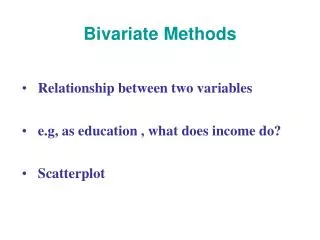
We are interested in studying the following problems: Q1: Are GPA’s different between male and female? • This is a comparative study • Graphical methods: side-by-side bar charts or pie charts, or stacked bar charts. • Numerical comparison between two independent groups. Q2: Is there a relationship between GPA and Hours study per week? • This is a relationship study • Graphical method: scatter plots between two variables. • Numerical investigation of correlation or regression models. Module One shows a variety of graphical and numerical summaries for comparative studies. In this module,We will focus on the relationship of bivariate and regression modeling.
How to display relationship between two variables – Scatter plots • Describing patterns shown in the following scatter plots: - What type of pattern do you see? Upward or downward? Curved? None or random? - How strong is the pattern? All points follow it? Only weakly visible? - Are there any unusual observations? Outliers? Clusters? Explanation for groupings?
Numerical Measures for Quantitative Bivariate Data • Numerical measurement to quantify the relation is the Pearson’s correlation coefficient, r. • Properties of r: -1 r 1 r = 1 means perfect positive correlation. Every pair of observation is on the linear line. r = -1: perfect negative correlation. r = 0: No correlation. A random pattern. • In most real world applications, r is rarely 1 , -1 or 0.
Positive correlation, outlier Random, no correlation Some common relationship patterns Y = b + ax a > 0. With or without the outlier, the regression models are different. r is positive, and around .7 with the outlier. Without the outlier, r would be close to one. Y = b + ax, with a almost zero. r is almost zero.
Nonlinear Positive linear, Nonlinear Y = b + ax with b about 19, a almost zero Y = b + ax +cx2 With c > 0, Y has a minimum r is about zero Y = b + ax with b about 23, a > 0 Y = b + ax +cx2 With c < 0 and Y has a maximum R is positive, and about .7
Highly positive Highly negative Y = b + ax b about 35, a < 0 r close to -1. Y = b + ax B about 20, a > 0 r close to one.
Numerical Measure of Relationship – Correlation Coefficient • A simple measure of the relationship between two variables x and y is the correlation coefficient, r: where sx and sy are the standard deviations for the variables x and y. • The new quantity sxy is called the covariance between x and y and is defined as: • A computing formula for the covariance: where Sxiyi is the sum of the products xiyi for each of the n pairs of measurements.
Some connections between correlation coefficient, r and • If the points in the x vs y plot tend to run from lower left to upper right, then and r will be positive. • If the points tend to run from upper left to lower right, then • and r will be negative. • If the points are scattered high and low and left and right, then and r will be close to zero. Use Minitab to compute the correlation coefficient, r: • Go to Stat, choose basic statistics, • choose Correlation, then enter the Dialog box. • If ‘Display p-value’ is selected, the output will show if the correlation coefficient is significant or not. (More will be discussed later).
In many real world applications, we are interested in determining the relationship between Y and X using a model for prediction purpose. E.g., How can you build a model to predict mileage using car weights? • The value of y typically depends on the value of x; y is called the dependent variable and x is called the independent variable. • Sometimes it is possible to describe the relationship relating x to y using a straight line given by the equation y = ax + b. • The best-fitting line relating y to x, called the regression or least-squares line, is found by minimizing the sum of the squared differences between the data points and the line itself. • In some cases, the relation between Y and X is nonlinear. The regression line is a polynomial regression, not a straight line. For example, a quadratic polynomial regression has the form: Y = ao + a1x + a2x2. The rice production and the amount of fertilizer would have such a relation.
In many situations, we would like to interpret the response Y using several independent variables x’s. This is what we call, Multiple Regression Model: Example, both temperature and humidity may have significant impact to the length of time period for keeping mea product fresh. An experiment can be conducted to measure the time period under different combination of (humidity, temperature). Y = time period the meat is fresh. X1 = humidity, X2 = temperature And a multiple regression model would be: Y = ao + a1X1 + a2X2 + a3(X1*X2) + a4X12 + a5X22. This model is also called Response Surface Model. Since our main purpose is to find the optimal combination of (humidity and temperature) that will maximize the time. In fact, we can make this experiment more complicated by adding different types of meat into the study. Modeling the time using humidity and temperature, at the same time, compare the time among different types of meat.This is a regression modeling involves with both quantitative and qualitative independent variables. Regression modeling itself is a series of two semester course. The discussion of this subject will be brief, due to the time limit.
The concept of the Least Squared Method for developing regression models:
The idea behind the regression model is to find the ‘Best line’ that interprets the relationship the most. One way to do to find the line that gives smallest sum of squared residuals. The term residual is the difference from the observed yi to the predicted yi. • More specifically, we first choose a type of model that we think will fit the relation best, in this case, it is y = a + bx, a straight line. In order to distinguish between observed data (xi, yi), we use the notation: • The the difference is . This is the residual for the ith case. • The best least squared regression model is the one that minimizes the sum of squared ei’s. • That is we are looking for a and b using the data (xi, yi) so that • is minimized. • The solution of this minimization problem gives the formulas for computing b and a: • When r is positive, b is positive; when r is negative, b is negative; when r is zero, b is zero.
Computing Regression Line similar to the above one for fitting GPA using Hours Study: • Go to Stat, choose Regression, select ‘Fitted Line Plot’. • In the Dialog box, enter GPA for Response Y, and Hourstudy for Predictor X. • You may choose a linear, a quadratic or cubic regression line, depending on the relation shown on the data. • You may click on ‘Options’, and choose to ‘Display Confidence Band’ as the above example shown.
A few key points about regression modeling 1. The regression model for this study is GPA = 2.15 + .15(Hours Study) 2. This model explains 38% of GPA information can be explained by the Hours Study. (R2(Adjusted) = .378). More specifically, R2 measures the proportion of variation of the GPA explained by the Hours Study. Generally speaking, the higher the R2, the more the X variable can explain the pattern of the response. 3. We can apply the model to estimate a student’s GPA if we know the # of hours they study per week. For example, Tom spends about 5 hours per week studying. Based on this model, we estimate his GPA would be about 2.9. 4. Further more, we are 95% confidence that if a student spends 5 hours per week to study, his/her GPA would be between 2.74 to 3.05. This interval is from the 95% confidence upper and lower bands shown on the graph.. It says: for a given X-value, the # of hours study, the range of the GPA will be within the given band with 95% of chance. Numerical bands can also be computed using Minitab.
5. What happen if a student spent , on average, 20 hours to study. What is the estimated GPA? Using the model, the estimate would be 5.15, which is impossible! So, what is wrong? 6. How do we know if the variable ‘Hours Study’ is indeed a ‘good’ predictor? The R2 gives some message about this. The higher the R2, the more the X variable can explain GPA, and therefore, the prediction will be more precise. Another commonly used approach to find out the degree of significance of an X variable is to conduct a hypothesis test. HOW?
Using Minitab for Regression Modeling • When we fit the regression line for the modeling GPA using Hours Study, we use ‘Fitted Line Plot’ procedure. This is only for one variable case with rather limited results. A more general procedure in Minitab for regression modeling is the following: • Go to Stat, choose Regression, then select ‘Regression’ procedure. • In the Dialog box, enter GPA as Response. Enter HourStudy into the Predictors box. (You can enter as many independent variables as needed here for multiple regression). • There are four sub-dialog boxes available: Graphs for residual analysis, Results for additional outputs, Storage for storing some results in the worksheet for further analysis, Options for a variety of additional analysis. • The confidence limit for studying 5 hours that I obtained (2.74 to 3.05) is computed in the Options Dialog. Click on the ‘Options’, enter the X values that you would like to compute confidence limits or prediction limits (in this case, I enter 5),and choose to store confidence limits. This will give us 2.74 and 3.05 in the data worksheet as CLIM1 and CLIM2.
How to conduct a complete Regression Analysis? The above discussion gives some basic regression modeling , and interpretations, and introduce Minitab to conduct these analysis. It will take some time to talk about a more complete regression analysis. If we have time, we will come back to this topic. Before we move onto other topic, let’s work on a project of simple linear regression analysis.