Download
1 / 36
360 likes | 475 Views
Numerics of Parametrization. ECMWF training course May 2006. by Nils Wedi ECMWF. Overview. Introduction to ‘physics’ and ‘dynamics’ in a NWP model from a numerical point of view Potential numerical problems in the ‘physics’ with large time steps

E N D
Numerics of Parametrization ECMWF training course May 2006 by Nils Wedi ECMWF
Overview • Introduction to ‘physics’ and ‘dynamics’ in a NWP model from a numerical point of view • Potential numerical problems in the ‘physics’ with large time steps • Coupling Interface within the ‘physics’ and between ‘physics’ and ‘dynamics’ • Concluding Remarks • References
Introduction... • ‘physics’, parametrization: “the mathematical procedure describing the statistical effect of subgrid-scale processes on the mean flow expressed in terms of large scale parameters”, processes are typically:vertical diffusion, orography, cloud processes, convection, radiation • ‘dynamics’: computation of all the other terms of the Navier-Stokes equations (eg. in IFS: semi-Lagrangian advection)
Introduction... • Goal: reasonably large time-step to save CPU-time without loss of accuracy • Goal: numerical stability • achieved by…treating part of the “physics” implicitly • achieved by… splitting “physics” and “dynamics” (also conceptual advantage)
Introduction... • Increase in CPU time substantial if the time step is reduced for the ‘physics’ only. • Iterating twice over a time step almost doubles the cost.
Introduction... • Increase in time-step in the ‘dynamics’ has prompted the question of accurate and stable numerics in the ‘physics’.
Potential problems... • Misinterpretation of truncation error as missing physics • Choice of space and time discretization • Stiffness • Oscillating solutions at boundaries • Non-linear terms • correct equilibrium if ‘dynamics’ and ‘physics’ are splitted ?
Equatorial nutrient trapping – example of ambiguity of (missing) “physics” or “numerics” observation • Effect of insufficient vertical resolution and the choice of the numerical (advection) scheme Model B Model A A. Oschlies (2000)
Discretization e.g. Tiedke mass-flux scheme Choose:
Discretization • Stability analysis, choose a solution: • Always unstable as above solution diverges !!!
Stiffness e.g. on-off processes, decay within few timesteps, etc.
Pic of stiffness here Stiffness: k = 100 hr-1, dt = 0.5 hr
Stiffness • No explicit scheme will be stable for stiff systems. • Choice of implicit schemes which are stable and non-oscillatory is extremely restricted.
Boundaries Classical diffusion equation, e.g. tongue of warm air cooled from above and below.
Pic of boundaries here T0=160C , z=1600m, k=20m2/s, dz=100m, cfl=k*dt/dz2
Non-linear terms e.g. surface temperature evolution
Pic of non-linear terms here predic-corr non-Linear terms: K=10, P=3
Coupling interface... • Splitting of some form or another seems currently the only practical way to combine “dynamics” and “physics” (also conceptual advantage of “job-splitting”) • Example: typical time-step of the IFS model at ECMWF (2TLSLSI)
Sequential vs. parallel splitvdif - dynamics A. Beljaars parallel split sequential split
Noise in the operational forecasteliminated through modified coupling
Splitting within the ‘physics’ ‘Steady state’ balance between different parameterized processes: globally P. Bechtold
Splitting within the ‘physics’ ‘Steady state’ balance between different parameterized Processes: tropics
Splitting within the ‘physics’ • “With longer time-steps it is more relevant to keep an accurate balance between processes within a single time-step” (“fractional stepping”) • A practical guideline suggests to incorporate slow explicit processes first and fast implicit processes last (However, a rigid classification is not always possible, no scale separation in nature!) • parametrizations should start at a full time level if possible otherwise implicitly time-step dependency introduced • Use of predictor profile for sequentiality
Splitting within the ‘physics’ Inspired by results! Previous operational: Choose: =0.5 (tuning) Currently operational: Predictor-corrector scheme by iterating each time step and use these predictor values as input to the parameterizations and the dynamics. Problems: the computational cost, code is very complex and maintenance is a problem, tests in IFS did not proof more successful than simple predictors, yet formally 2nd order accuracy may be achieved ! (Cullen et al., 2003, Dubal et al. 2006)
Concluding Remarks • Numerical stability and accuracy in parametrizations are an important issue in high resolution modeling with reasonably large time steps. • Coupling of ‘physics’ and ‘dynamics’ will remain an issue in global NWP. Solving the N.-S. equations with increased resolution will resolve more and more fine scale but not down to viscous scales: averaging required! • Need to increase implicitness (hence remove “arbitrary” sequentiality of individual physical processes, e.g. solve boundary layer clouds and vertical diffusion together) • Other forms of coupling are to be investigated, e.g. embedded cloud resolving models and/or multi-grid solutions (solving the physics on a different grid; a finer physics grid averaged onto a coarser dynamics grid can improve the coupling, a coarser physics grid does not !) (Mariano Hortal, work in progress)
References • Dubal M, N. Wood and A. Staniforth, 2006. Some numerical properties of approaches to physics-dynamics coupling for NWP. Quart. J. Roy. Meteor. Soc., 132, 27-42. • Beljaars A., P. Bechtold, M. Koehler, J.-J. Morcrette, A. Tompkins, P. Viterbo and N. Wedi, 2004. Proceedings of the ECMWF seminar on recent developments in numerical methods for atmosphere and ocean modelling, ECMWF. • Cullen M. and D. Salmond, 2003. On the use of a predictor corrector scheme to couple the dynamics with the physical parameterizations in the ECMWF model. Quart. J. Roy. Meteor. Soc., 129, 1217-1236. • Dubal M, N. Wood and A. Staniforth, 2004. Analysis of parallel versus sequential splittings for time-stepping physical parameterizations. Mon. Wea. Rev., 132, 121-132. • Kalnay,E. and M. Kanamitsu, 1988. Time schemes for strongly nonlinear damping equations. Mon. Wea. Rev., 116, 1945-1958. • McDonald,A.,1998. The Origin of Noise in Semi-Lagrangian Integrations. Proceedings of the ECMWF seminar on recent developments in numerical methods for atmospheric modelling, ECMWF. • Oschlies A.,2000. Equatorial nutrient trapping in biogeochemical ocean models: The role of advection numerics, Global Biogeochemical cycles, 14, 655-667. • Sportisse, B., 2000. An analysis of operator splitting techniques in the stiff case. J. Comp. Phys., 161, 140-168. • Wedi, N., 1999. The Numerical Coupling of the Physical Parameterizations to the “Dynamical” Equations in a Forecast Model. Tech. Memo. No.274 ECMWF.