Download
1 / 17
170 likes | 299 Views
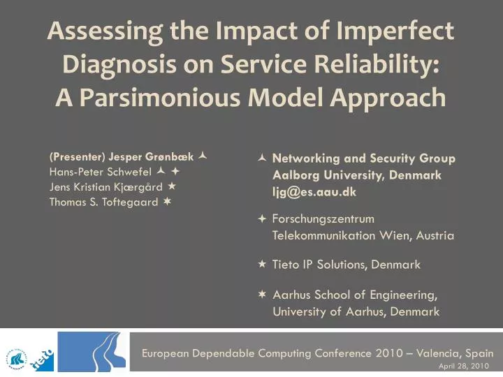
(Presenter) Jesper Grønbæk Hans-Peter Schwefel Jens Kristian Kjærgård Thomas S. Toftegaard . Networking and Security Group Aalborg University, Denmark ljg@es.aau.dk. . Forschungszentrum Telekommunikation Wien, Austria.

E N D
(Presenter) Jesper Grønbæk Hans-Peter Schwefel Jens KristianKjærgård Thomas S. Toftegaard Networking and Security Group Aalborg University, Denmark ljg@es.aau.dk ForschungszentrumTelekommunikation Wien, Austria Assessing the Impact of Imperfect Diagnosis on Service Reliability:A Parsimonious Model Approach Tieto IP Solutions, Denmark Aarhus School of Engineering, University of Aarhus, Denmark < European Dependable Computing Conference 2010 – Valencia, Spain April 28, 2010
Imperfect Diagnosis • Conclusions Background and Motivation • Network fault diagnosis • Dependable end-user service provisioning in Next Generation Network architectures Dominated by wireless networks, mobility and varying traffic conditions • Challenged by unreliable observations and hidden network states • Imperfect Diagnosis • Modelling imperfect diagnosis • Goals of modelling • Determine best remediation actions • Determine best trade-off of imperfections • Assess properties of a given diagnosis component (function level modelling[1], system level simulation [2]) • Light-weight models desirable for frequent model re-evaluations
Imperfect Diagnosis • Conclusions Example: DecentalizedFault Management Framework • ODDR decentralized fault management framework [3] [4](Observation, Diagnosis, Decision and Remediation) • End-node Driven Fault Management • Joint view on imperfect diagnosis and decisions (remediation, observation collection ) • Operation in dynamic environment frequent model re-evaluations Subsequent focus on trade-off of imperfections (best diagnosis settings)
Background on Diagnosis Approaches • Conclusions Definitions of Diagnosis Outcomes • Diagnosis atomic view • Single observation • Two network states (Normal/Fault) • Discrete diagnosis steps (period T) • Generic Diagnosis (state estimation) definitions
Background on Diagnosis Approaches • Conclusions Diagnosis Classes • Two levels of complexity of diagnosis behaviour • One-shot1: diagnosis estimate based on a single set of observations in time • No correlation of diagnosis estimates from diagnosis Simple model representation proposed in [3] • Over-time1: diagnosis estimate based on new and old observations • Means to improve diagnosis estimates • Strong correlation added by diagnosis component • Comparison • One-shot: threshold on round-trip time (RTT) • Over-time: -count heuristic (Bondavalli et al. [1]) on one-shot estimates • Transient effects from network neglected • Over-time has highly transient phase; yet significant improvement • Identify best trade-off: Reaction Time & False Alarms • Simple parameterization from steady-state behaviour is difficult 2000 repetitions 1Terminologyadapted from [5]
Parsimonious Diagnosis Model • Conclusions Definition and Parameters • Four-state Markov model presented in [3] • Controlled by geometric ON-OFF network state process (fault/repair occurence) {pf, pr} • 2 free parameters {P(TN|Ns=Normal) = TNR = (1-FPR), P(TP|Ns=Fault) = TPR = (1-FNR)} • Explore model capabilities • Remediation assumption: fail-over on network fault state diagnosis • 6 free parameters • fixed {pf, pr} 4 free parameters System Equations
Parsimonious Diagnosis Model • Conclusions Diagnosis Metrics Definitions • Diagnosis Metrics • Proposed Metrics (steady state) • Probability on Remediation on False Alarm, (pRFA) • Mean Remediation Reaction Time (mRRT) Note, two parameters and four free • Diagnosis Trace • Start diagnosis in normal network state for a given set {pf, pr} • Observe until alarm is diagnosed • Perform M repetitions and derive O=#FA • pRFA= O/M • mRRT, mean time to remediation over all M
Parsimonious Diagnosis Model • Conclusions Diagnosis Metrics Equations • Closed-form equations derived by linear algebraic approaches [6] • Probability on Remediation on False Alarm (pRFA) Probability of absorption • Mean Remediation Reaction Time (mRRT) Mean time to absorption • Solving yields two linear equations: Initial state Absorbingstates
Parameterization by Diagnosis Metrics • Conclusions • Underdetermined problem solved by heuristics (MI) Minimize pFPTN and pTPFN.Minimize direct transitions TNFP and FNTP • Behaviour in transient analysis: • Initial study parameters: T = 0.4s, Mean normal period= 12.42s, Mean fault period = 15 s • Captures an initial higher probability of pRTAover all alarms (pRTA+pRFA) pRFA minimize pRTA (pRFA + pRTA) pRTA minimize
Case: Time Constrained Data Transfer • Conclusions Background • QoS requirement: Complete SCTP based file transfer within tdeadline seconds with the probability: W • Fault: Congestion in operator infrastructure (occurrence and repair, ON-OFF model) • Remediation: Single fail-over from network A to network B • Diagnosis: Simple threshold based on RTT and a-count • Decision: Fail-over on network fault state diagnosis
File Transfer Completion Time CDF Case: Time Constrained Data Transfer • Conclusions Policy Evaluation Model • Policy Evaluation Discrete Time Markov Model (PE DTMC) [3] • State Space: SPE = {Activenetwork, Time progress, File progress, Network state, Diagnosisstate} • Ωmodel = ΣSPEss(r, n) m r =1
Model Sensitivity Analysis • Conclusions • Model based sensitivity analysis on Ω • Vary mRTTand pRFA, tdeadline = 30s & filesize=10 MByte • Compare to perfect diagnosis and no-failover policy • Both metrics have a clear impact on Ω, mRTT promptness and pRFA-> correctness • Most sensitive to high pRFA wrong fail-over cannot be remediated • Can deliver significantly worse performance than no fail-over PerfectDiagnosis Nofail-over
Reliability Evaluation Results • Conclusions Background & Trade-off Results • Study properties of a-count diagnosis component • a-count controlled by two parameters: k forgetting factor, aT threshold • PE DTMC Model based analysis • Simulation basedanalysis • System level simulation basedon ns-2 • Provideevaluation of W and traces of diagnosis performance • Considertwosettings of one-shotdiagnosis: • Tradeoff options of a-count (obtained from single trace set, 2000 runs) g0 = (TPR, TNR) = (0.983, 0.097) g1= (TPR, TNR) = (0.953, 0.225)
Reliability Evaluation Results • Conclusions Background & Trade-off Results • PE DTMC model basedanalysis • Simple threshold • g0 performsbetterthang1 (as shown in [3]) • a-count • Overall leads to improvement filtering out false alarms • Optimal settingsexist • g1: k=0.92, aT=2.5leads to bestresults Obtainablereduction of pRFAwithoutsimilarincrease in mRTT • Simulation basedanalysis • Consistentconclusions to model • Qualitative differences • stochastic time model • Simplified data-transfer model Wmodel ThresholdaT Simple threshold Wsimulation ThresholdaT
Conclusion & Outlook • Conclusions • Conclusions • Proposed parsimonious imperfect diagnosis model for light-weight assessment of best diagnosis component settings; also considering complex class of over-time diagnosis components • Defined representative imperfect diagnosis performance metrics and derived their closed-form equations in the model • Presented service reliability case and performed model based sensitivity analysis of reliability on imperfect diagnosis performance metrics • Used model to assess diagnosis performance properties of over-time diagnosis heuristic from literature and define best setting • Shown by system level simulation analysis that diagnosis model can capture essential imperfect diagnosis performance characteristics • Outlook • Introduce more complex decision policies • Application state information minimize remediation • Multiple fault diagnosis • Decisions to collect more information Need to study diagnosis model behaviour after positive diagnosis and potentially extend
DRCN 09 - Washington DC Questions & Discussion • Conclusions
References [1] Threshold-based mechanisms to discriminate transient from intermittent faults. A. Bondavalli, S. Chiaradonna, F. Di Giandomenico, and F. Grandoni, IEEE Transactions on Computers, vol. 49, no. 3, pp. 230–245, 2000. [2] Probabilistic Fault-Diagnosis in Mobile Networks Using Cross-Layer Observations. A. Nickelsen, J. Grønbæk, T. Renier, and H.-P. Schwefel, “” In Proceedings of AINA 09, pp. 225–232, 2009. [3] Model based evaluation of policies for end-node driven fault recovery. J. Grønbæk, H.-P. Schwefel, and T. Toftegaard, Proc. DRCN 09, 2009. [4] Towards self-adaptive reliable network services in highly-uncertain environments. A. Ceccarelli, J. Grønbæk, L. Montecchi, A. Bondavalli, and H. P. Schwefel, To appear in proceedings of WORNUS 10, May, 2010. [5] HiddenMarkov Models as a Support for Diagnosis: Formalization of the Problem and Synthesis of the Solution. A. Daidone, F. Di Giandomenico, S. Chiaradonna, and A. Bondavalli, in 25th IEEE Symposium onReliableDistributed Systems, 2006. SRDS’06, 2006, pp. 245–256. [6] Queueing Theory – A Linear Algebraic Approach. L. Lipsky, 2nd ed. Springer, 2009. ,,