Download
1 / 72
720 likes | 873 Views
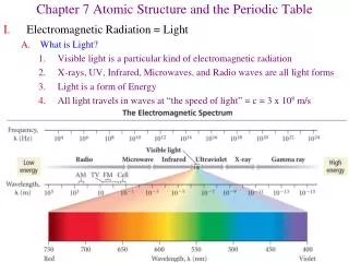
Chapter 7 Atomic Structure and the Periodic Table.

E N D
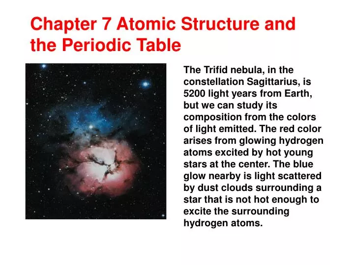
Chapter 7 Atomic Structure andthe Periodic Table The Trifid nebula, in the constellation Sagittarius, is 5200 light years from Earth, but we can study its composition from the colors of light emitted. The red color arises from glowing hydrogen atoms excited by hot young stars at the center. The blue glow nearby is light scattered by dust clouds surrounding a star that is not hot enough to excite the surrounding hydrogen atoms.
Assignment for Chapter 7 18, 27, 33, 43, 55, 65
Comte’s Agnosticism (unknowablism)“We will never know anything about the stars because we cannot get to them.”
Figure 7.1 (a) In a spectrometer, the light emitted by an energetically excited sample of an element is passed through a slit, to give a narrow ray, and then through a prism. The prism separates the ray into different colors, which are recorded photographically. The spectral lines on the photograph are the separate images of the slit. Spectroscopy is the most important tool for studying atomic and molecular structure.
Figure 7.1 (b) A rainbow is formed when white light from the Sun is split into its component colors by raindrops that act as tiny prisms. The light enters the front of the raindrop, reflects from the back, and emerges from the front. Double rainbows are formed when the light reflects a second time inside the drop.
Figure 7.2 The electric field of electromagnetic radiation oscillates in space and time. The length of an arrow at any point at a given instant represents the strength of the force that the field exerts on a charged particle at that point. Note the wavelike distribution of the field. c is a constant for all electromagnetic waves
Figure 7.3 The color of electromagnetic radiation is determined by its wavelength (and frequency). (a) The wavelengths of the three rays shown here are drawn to scale and you can see that the wavelengths of green, yellow, and red light increase in that order. The perception of color arises from the effect of the radiation on our eyes and the response of our brain. (b) Each lamp in a traffic signal generates white light, a mixture of all colors, but the tinted glass screens allow only certain wavelengths to pass through. (b)
Figure 7.4 This diagram represents a “snapshot” of an electromagnetic wave at a given instant. The distance between the peaks is the wavelength of the radiation. The amplitude (height) of the peaks depends on the intensity of the radiation.
Figure 7.5 Wavelength and frequency are inversely related. The two parts of this illustration show the electric field at three instants that you might experience as a single wave flashed by a single point at the speed of light from left to right. The position of the wave at the first instant is the light gray wave and its position at the third instant is the blue wave. (a) Short-wavelength radiation: note how the electric field changes markedly at the three successive instants. (b) For the same three instants, the electric field of the long-wavelength radiation changes much less. Short-wavelength radiation has a high frequency, whereas long-wavelength radiation has a low frequency.
Figure 7.6 The electromagnetic spectrum and the names of its regions. Note that the region we call “visible light” occupies a very narrow range of wavelengths. The regions are not shown to scale.
Figure 7.7 When a metal is illuminated with light, electrons are ejected, provided the frequency is above a threshold frequency that is characteristic of the metal. Radiation with a lower frequency will not cause electrons to be ejected, no matter how intense it is. Wave theory of light cannot explain photoelectric effect! Light must consist of photons (quantum of light).
Figure 7.8 The red glow from this hydrogen discharge lamp comes from excited hydrogen atoms that are returning to a lower energy state and emitting the excess energy as visible radiation.
Figure 7.9 The spectrum of atomic hydrogen. The spectral lines have been assigned to various groups of similar wavelength called series; the Balmer and Lyman series are shown here. Each line corresponds to a photon emit by an electron “jumping” from higher energy level to the ground state Discrete spectral lines imply discrete structure of electronic energy
Figure 7.10 When an atom undergoes a transition from a state of higher energy to one of lower energy, it loses energy that is carried away as a photon. The greater the energy loss, the higher the frequency (and the shorter the wavelength) of the radiation emitted. Thus, transition A generates light with a higher frequency and shorter wavelength than transition B.
Figure 7.11 The spectrum of atomic hydrogen (reproduced on the right) tells us the arrangement of the energy levels of the atom because the frequency of the radiation emitted in a transition is proportional to the energy difference between the two energy levels involved. The 0 on the energy scale corresponds to the completely separated proton and electron. The numbers on the right label the energy levels: they are examples of quantum numbers (see Section 7.7).
Figure 7.12 When a guitar string vibrates, only certain wavelengths can be sustained over time—those for which the amplitude of the wave goes to 0 at each end. One or more complete half-wavelengths must fit exactly between the end points. (a) A guitar string at rest. (b) One-half wavelength. (c) One full wavelength.
Wave-Particle Duality All particles show wavelike properties All waves have particle behaviors
Figure 7.13 Davisson and Germer showed that electrons give a diffraction pattern when reflected from a crystal. G. P. Thomson working in Aberdeen, Scotland showed that they also give a diffraction pattern when they pass through a very thin gold foil. The latter is shown here. G. P. Thomson was the son of J. J. Thomson, who identified the electron (Section 1.3). Both received Nobel prizes, J. J. for showing that the electron is a particle and G. P. for showing that it is a wave.
Figure 7.14 (a) In classical mechanics, a particle follows a path, or trajectory, and its position can be predicted at any instant. (b) In quantum mechanics, the particle is distributed like a wave, so its location cannot be predicted exactly. Where the wavefunction has a high amplitude, there is a high probability of finding the particle; where the amplitude is low, there is only a small probability of finding the particle.
Figure 7.15 Erwin Schrödinger (1887–1961). The Schrödinger equation is shown superimposed on Schrödinger’s head. The constant stands for h /2. Electrons are waves inside an atom. …..not particles. They don’t believe me…I quit! Erwin Schrödinger, 1000 Austrian Schilling (1983)
Figure 7.16 The Born interpretation of a wavefunction. The probability of the electron being found at a point is proportional to the square of the wavefunction (indicated by 2), as depicted by the density of shading in the band below. Note that the probability density is 0 at a node. A node is a point where the wavefunction passes through 0, not merely approaches 0. Wave = wave of probability
Figure 7.17 The three-dimensional electron cloud corresponding to an electron in the lowest energy state of hydrogen. This wavefunction is called the 1s-orbital (Section 7.7). The density of shading represents the probability of finding the electron at any point. The superimposed graph shows how the probability varies with the distance from the nucleus along any radius. Cloud = cloud of probability
Figure 7.18 The simplest way of drawing an atomic orbital is as a boundary surface, a surface within which there is a high probability (typically, 90%) of finding the electron. The spheres here represent the boundary surfaces of the s-orbitals in the first three energy levels. Note that s-orbitals with n > 1 have internal spherical nodes and that the size of the orbital increases with n. We shall use blue to denote s-orbitals, but that color is only an aid to their identification. These s-orbitals are waves.
Figure 7.19 The boundary surface of a p-orbital has two lobes; the nucleus lies on the plane that divides the two lobes, and an electron will, in fact, never be found at the nucleus itself if it is in a p-orbital. There are three p-orbitals of a given energy, and they lie along three perpendicular axes. We shall use yellow to indicate p-orbitals. Note that the orbital has opposite signs (as depicted by the depth of color) on each side of the nodal plane. These p-orbitals are waves.
Figure 7.20 The boundary surface of a d-orbital is more complicated than that of an s- or a p-orbital. There are five d-orbitals of a given energy; four of them have four lobes; one is slightly different. In each case, an electron that occupies a d-orbital will not be found at the nucleus. We shall use orange to indicate d-orbitals, with different depths of color to indicate different signs. These d-orbitals are waves.
Figure 7.21 The boundary surface of one of the seven f-orbitals of a shell (with n 4). The f-orbitals have a complex appearance. Their shapes will not be needed again in this text. However, their existence is important for understanding the periodic table, the presence of the lanthanides and actinides, and the properties of the later d-block elements. This f-orbital is a wave.
All f-orbitals These f-orbitals are waves.
Figure 7.22 The permitted energy levels of a hydrogen atom as calculated from Eq. 6. The 0 on the energy scale corresponds to the completely separated proton and electron; the lowest energy state lies at hRH below the 0 of energy. The levels are labeled with the principal quantum number, n, which ranges from 1 (for the lowest state) to infinity (for the separated proton and electron). Compare this diagram with the experimentally determined array of levels shown in Fig. 7.11.
Figure 7.23 A summary of the arrangement of shells, subshells, and orbitals in an atom and the corresponding quantum numbers. Note that the quantum number ml is an alternative label for the individual orbitals: in chemistry, it is more common to use x, y, and z as labels, as shown in Figs. 7.19 and 7.20. There is no direct correspondence between axis designation and the numerical value of ml.
Figure 7.24 The solution to Example 7.5. The boxes represent the individual orbitals in each subshell. There are 16 orbitals in the shell with n= 4, each of which can hold two electrons. The atomic orbitals for n=4
Investigating Matter 7.1 The quantization of electron spin is confirmed by the Stern-Gerlach experiment, in which a stream of atoms splits into two as it passes between the poles of a magnet. The atoms in one stream have an odd electron, and those in the other an odd electron.
Figure 7.25 The two spin states of an electron can be represented as clockwise or counterclockwise rotation around an axis passing through the electron. The two states are labeled by the quantum number ms and depicted by the arrows shown on the right.
7.9 The Electronic Structure of Hydrogen Free electron state 3p 3,1,1,1/2 3,1,1,-1/23,1,0,1/2 3,1,0,-1/2 3,1,-1,1/2 3,1,-1,-1/2 3s 3,0,0,1/2 3,0,0,-1/2 2p 2,1,1,1/2 2,1,1,-1/2 2,1,0,1/2 2,1,0,-1/2 2,1,-1,1/2 2,1,-1,-1/2 2s 2,0,0,1/2 2,1,1,-1/2 1s 1,0,0,1/2 1,0,0,-1/2 Ionization energy=hRH=2x10-18J
Lithium Sodium Potassium Rubidium
The Building-up Principle Pauli’s Exclusion Principle: No more than two electrons may occupy any given orbital. When two electrons do occupy one orbital, their spins must be paired. Hund’s Rule: If more than one orbital in a subshell is available, electrons will fill empty orbitals before pairing on one of them. Ground state (configuration)
Z Z Z Consequences of Electron-Electron Interactions Orbital energy: Electron-Nucleuspull (attractive) Electron-Electronpush(repulsive) Shielding: The attraction is reduced because of the presence of other electrons Zeff < Z Penetration:s-electrons get very close to the nucleus, reducing their energy Zeff = Z-S The “trajectories” of s-electrons (penetration)
Orbital Energy Crossing For atoms with Z>20, energy crossing (typically a 4s-electron has lower energy than a 3d electron— against the building-up principle) occurs because shielding increases the energy of non-s-electrons in outer shells whereas penetration reduces the energy of s-electrons.
Periodical Table Dmitri Ivanovich Mendeleev (1834-1907)