Download
1 / 78
780 likes | 900 Views
Simulation Techniques: Outline. Lecture 1: Introduction: Statistical Mechanics, ergodicity, statistical errors.

E N D
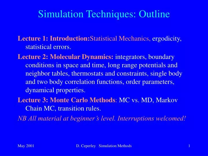
Simulation Techniques: Outline Lecture 1: Introduction:Statistical Mechanics, ergodicity, statistical errors. Lecture 2: Molecular Dynamics: integrators, boundary conditions in space and time, long range potentials and neighbor tables, thermostats and constraints, single body and two body correlation functions, order parameters, dynamical properties. Lecture 3: Monte Carlo Methods: MC vs. MD, Markov Chain MC, transition rules. NB All material at beginner’s level. Interruptions welcomed! D. Ceperley Simulation Methods
Introduction to Simulation:Lecture 1 • Why do simulations? • Some history • Review of statistical mechanics • Newton’s equations and ergodicity • The FPU “experiment” • How to get something from simulations: statistical errors D. Ceperley Simulation Methods
Why do simulations? • Simulations are the only general method for “solving” many-body problems. Other methods involve approximations and experts. • Experiment is limited and expensive. Simulations can complement the experiment. • Simulations are easy even for complex systems. • They scale up with the computer power. D. Ceperley Simulation Methods
Two Simulation Modes A. Give us the phenomena and invent a model to mimic the problem. The semi-empirical approach. But one cannot reliably extrapolate the model away from the empirical data. B. Maxwell, Boltzmann and Schoedinger gave us the model. All we must do is numerically solve the mathematical problem and determine the properties. (first principles or ab initio methods) This is what we will talk about. D. Ceperley Simulation Methods
“The general theory of quantum mechanics is now almost complete. The underlying physical laws necessary for the mathematical theory of a large part of physics and the whole of chemistry are thus completely known, and the difficulty is only that the exact application of these laws leads to equations much too complicated to be soluble.” Dirac, 1929 D. Ceperley Simulation Methods
Challenges of Simulation Physical and mathematical underpinings: • What approximations come in: • Computer time is limitedfew particles for short periods of time. (space-time is 4d. Moore’s Law implies lengths and times will double every 6 years if O(N).) • Systems with many particles and long time scales are problematical. • Hamiltonian is unknown, until we solve the quantum many-body problem! • How do we estimate errors? Statistical and systematic. • How do we manage ever more complex codes? D. Ceperley Simulation Methods
Short history of Molecular Simulations • Metropolis, Rosenbluth, Teller (1953) Monte Carlo Simulation of hard disks. • Fermi, Pasta Ulam (1954) experiment on ergodicity • Alder & Wainwright (1958) liquid-solid transition in hard spheres. “long time tails” (1970) • Vineyard (1960) Radiation damage using MD • Rahman (1964) liquid argon, water(1971) • Verlet (1967) Correlation functions, ... • Andersen, Rahman, Parrinello (1980) constant pressure MD • Nose, Hoover, (1983) constant temperature thermostats. • Car, Parrinello (1985) ab initio MD. D. Ceperley Simulation Methods
Molecular Dynamics (MD) • Pick particles, masses and potential. • Initialize positions and momentum. (boundary conditions in space and time) • Solve F = m a to determine r(t), v(t). Newton (1667-87) • Compute properties along the trajectory • Estimate errors. • Try to use the simulation to answer physical questions. D. Ceperley Simulation Methods
What are the forces? • Crucial since V(q) determines the quality of result. • In this lecture we will use semi-empirical potentials: potential is constructed on theoretical grounds but using some experimental data. • Common examples are Lennard-Jones, Coulomb, embedded atom potentials. They are only good for simple materials. We will not discuss these potentials for reasons of time. • The ab initio philosophy is that potentials are to be determined directly from quantum mechanics as needed. • But computer power is not yet adequate in general. • A powerful approach is to use simulations at one level to determine parameters at the next level. D. Ceperley Simulation Methods
Statistical Ensembles • Classical phase space is 6N variables (pi, qi) and a Hamiltonian function H(q,p,t). • We may know a few constants of motion such as energy, number of particles, volume... • Ergodic hypothesis: each state consistent with our knowledge is equally “likely”; the microcanonical ensemble. • Implies the average value does not depend on initial conditions. • A system in contact with a heat bath at temperature T will be distributed according to the canonical ensemble: exp(-H(q,p)/kBT )/Z • The momentum integrals can be performed. • Are systems in nature really ergodic? Not always! D. Ceperley Simulation Methods
Ergodicity • Fermi- Pasta- Ulam “experiment” (1954) • 1-D anharmonic chain: V= [(q i+1-q i)2+ (q i+1-q i)3] • The system was started out with energy with the lowest energy mode. Equipartition would imply that the energy would flow into the other modes. • Systems at low temperatures never come into equilibrium. The energy sloshes back and forth between various modes forever. • At higher temperature many-dimensional systems become ergodic. • Area of non-linear dynamics devoted to these questions. D. Ceperley Simulation Methods
Let us say here that the results of our computations were, from the beginning, surprising us. Instead of a continuous flow of energy from the first mode to the higher modes, all of the problems show an entirely different behavior. … Instead of a gradual increase of all the higher modes, the energy is exchanged, essentially, among only a certain few. It is, therefore, very hard to observe the rate of “thermalization” or mixing in our problem, and this wa s the initial purpose of the calculation. Fermi, Pasta, Ulam (1954) D. Ceperley Simulation Methods
Equivalent to exponential divergence of trajectories, or sensitivity to initial conditions. (This is a blessing for numerical work. Why?) • What we mean by ergodic is that after some interval of time the system is any state of the system is possible. • Example: shuffle a card deck 10 times. Any of the 52! arrangements could occur with equal frequency. • Aside from these mathematical questions, there is always a practical question of convergence. How do you judge if your results converged? There is no sure way. Why? Only “experimental” tests. • Occasionally do very long runs. • Use different starting conditions. • Shake up the system. • Compare to experiment. D. Ceperley Simulation Methods
Statistical ensembles • (E, V, N) microcanonical, constant volume • (T, V, N) canonical, constant volume • (T, P N) constant pressure • (T, V , ) grand canonical • Which is best? It depends on: • the question you are asking • the simulation method: MC or MD (MC better for phase transitions) • your code. • Lots of work in last 2 decades on various ensembles. D. Ceperley Simulation Methods
Definition of Simulation • What is a simulation? An internal state “S” A rule for changing the state Sn+1 = T (Sn) We repeat the iteration many time. • Simulations can be • Deterministic (e.g. Newton’s equations=MD) • Stochastic (Monte Carlo, Brownian motion,…) • Typically they are ergodic: there is a correlation time T. for times much longer than that, all non-conserved properties are close to their average value. Used for: • Warm up period • To get independent samples for computing errors. D. Ceperley Simulation Methods
Problems with estimating errors • Any good simulation quotes systematic and statistical errors for anything important. • Central limit theorem: after “enough” averaging, any statistical quantity approaches a normal distribution. • One standard deviation means 2/3 of the time the correct answer is within of the estimate. • Problem in simulations is that data is correlated in time. It takes a “correlation” time to be “ergodic” • We must throw away the initial transient and block successive parts to estimate the mean value and error. • The error and mean are simultaneously determined from the data. We need at least 20 independent data points. D. Ceperley Simulation Methods
Estimating Errors • Trace of A(t): • Equilibration time. • Histogramof values of A ( P(A) ). • Meanof A (a). • Variance of A ( v ). • estimate of the mean: A(t)/N • estimate of the variance, • Autocorrelation of A (C(t)). • Correlation time (k ). • The (estimated)error of the (estimated) mean(s ). • Efficiency [= 1/(CPU time * error 2)] D. Ceperley Simulation Methods
Data Spork Interactive code to perform statistical analysis of data Shumway, Draeger,Ceperley D. Ceperley Simulation Methods
Statistical thinking is slippery • “Shouldn’t the energy settle down to a constant” • NO. It fluctuates forever. It is the overall mean which converges. • “My procedure is too complicated to compute errors” • NO. Run your whole code 10 times and compute the mean and variance from the different runs • “The cumulative energy has converged”. • BEWARE. Even pathological cases have smooth cumulative energy curves. • “Data set A differs from B by 2 error bars. Therefore it must be different”. • This is normal in 1 out of 10 cases. D. Ceperley Simulation Methods
Molecular Dynamics:Lecture 2 • What to choose in an integrator • The Verlet algorithm • Boundary Conditions in Space and time • Neighbor tables • Long ranged interactions • Thermostats • Constraints D. Ceperley Simulation Methods
Criteria for an Integrator • simplicity (How long does it take to write and debug?) • efficiency (How fast to advance a given system?) • stability (what is the long-term energy conservation?) • reliability (Can it handle a variety of temperatures, densities, potentials?) • compare statistical errors (going as h-1/2 ) with time step errors which go as hp where p=2,3...? D. Ceperley Simulation Methods
Characteristics of simulations. • Potentials are highly non-linear with discontinuous higher derivatives either at the origin or at the box edge. • Small changes in accuracy lead to totally different trajectories. (the mixing or ergodic property) • We need low accuracy because the potentials are not very realistic. Universality saves us: a badly integrated system is probably similar to our original system. This is not true in the field of non-linear dynamics or, in studying the solar system • CPU time is totally dominated by the calculation of forces. • Memory limits are not too important. • Energy conservation is important; roughly equivalent to time-reversal invariance.: allow 0.01kT fluctuation in the total energy. D. Ceperley Simulation Methods
The Verlet Algorithm The nearly universal choice for an integrator is the Verlet (leapfrog) algorithm r(t+h) = r(t) + v(t) h + 1/2 a(t) h2 + b(t) h3 + O(h4) Taylor expand r(t-h) = r(t) - v(t) h + 1/2 a(t) h2 - b(t) h3 + O(h4) Reverse time r(t+h) = 2 r(t) - r(t-h) + a(t) h2 + O(h4) Add v(t) = (r(t+h) - r(t-h))/(2h) + O(h2) estimate velocities Time reversal invariance is built in the energy does not drift. 8 1 2 3 4 5 6 7 9 10 11 12 13 D. Ceperley Simulation Methods
How to set the time step • Adjust to get energy conservation to 1% of kinetic energy. • Even if errors are large, you are close to the exact trajectory of a nearby physical system with a different potential. • Since we don’t really know the potential surface that accurately, this is satisfactory. • Leapfrog algorithm has a problem with round-off error. • Use the equivalent velocity Verlet instead: r(t+h) = r(t) +h [ v(t) +(h/2) a(t)] v(t+h/2) = v(t)+(h/2) a(t) v(t+h)=v(t+h/2) + (h/2) a(t+h) D. Ceperley Simulation Methods
Higher Order Methods? Statistical error for fixed CPU time. • Higher order does not mean better • Problem is that potentials are not analytic • Systematic errors • study from Berendsen 86 D. Ceperley Simulation Methods
Spatial Boundary Conditions Important because spatial scales are limited. What can we choose? • No boundaries; e.g. droplet, protein in vacuum. If droplet has 1 million atoms and surface layer is 5 atoms thick 25% of atoms are on the surface. • Periodic Boundaries: most popular choice because there are no surfaces (see next slide) but there can still be problems. • Simulations on a sphere • External potentials • Mixed boundaries (e.g. infinite in z, periodic in x and y) D. Ceperley Simulation Methods
Periodic Boundary Conditions Is the system periodic or just an infinite array of images? How do you calculate distances in a periodic system? D. Ceperley Simulation Methods
Periodic distances Minimum Image Convention: take the closest distance:|r|M = min ( r+nL) • Potential is cutoff so that V(r)=0 for r>L/2 since force needs to be continuous. How about the derivative? • Image potential VI = v(ri-rj+nL) • For long range potential this leads to the Ewald image potential. You need a back ground and convergence method (more later) -L -L/2 0 L/2 L x D. Ceperley Simulation Methods
Complexity of Force Calculations • Complexity is defined as how a computer algorithm scales with the number of degrees of freedom (particles) • Number of terms in pair potential is N(N-1)/2 O(N2) • For short range potential you can use neighbor tables to reduce it to O(N) • (Verlet) neighbor list for systems that move slowly • bin sort list (map system onto a mesh and find neighbors from the mesh table) • Long range potentials with Ewald sums are O(N3/2) but Fast Multipole Algorithms are O(N) for very large N. D. Ceperley Simulation Methods
! Loop over all pairs of atoms. do i=2,natoms do j=1,i-1 !Compute distance between i and j. r2 = 0 do k=1,ndim dx(k) = r(k,i) - r(k,j) !Periodic boundary conditions. if(dx(k).gt. ell2(k)) dx(k) = dx(k)-ell(k) if(dx(k).lt.-ell2(k)) dx(k) = dx(k)+ell(k) r2 = r2 + dx(k)*dx(k) enddo !Only compute for pairs inside radial cutoff. if(r2.lt.rcut2) then r2i=sigma2/r2 r6i=r2i*r2i*r2i !Shifted Lennard-Jones potential. pot = pot+eps4*ri6*(ri6-1)- potcut !Radial force. rforce = eps24*r6i*r2i*(2*r6i-1) do k = 1 , ndim force(k,i)=force(k,i) + rforce*dx(k) force(k,j)=force(k,j) - rforce*dx(k) enddo endif enddo enddo LJ Force Computation D. Ceperley Simulation Methods
Constant Temperature MD • Problem in MD is how to control the temperature. (BC in time.) • How to start the system? (sample velocities from a Gaussian distribution) If we start from a perfect lattice as the system becomes disordered it will suck up the kinetic energy and cool down. (v.v for starting from a gas) • QUENCH method. Run for a while, compute kinetic energy, then rescale the momentum to correct temperature, repeat as needed. • Nose-Hoover Thermostat controls the temperature automatically by coupling the microcanonical system to a heat bath • Methods have non-physical dynamics since they do not respect locality of interactions. Such effects are O(1/N) D. Ceperley Simulation Methods
Quench method • Run for a while, compute kinetic energy, then rescale the momentum to correct temperature, repeat as needed. • Control is at best O(1/N) D. Ceperley Simulation Methods
Nose-Hoover thermostat • MD in canonical distribution (TVN) • Introduce a friction force (t) SYSTEM T Reservoir Dynamics of friction coefficient to get canonical ensemble. Feedback restores makes kinetic energy=temperature Q= “heat bath mass”. Large Q is weak coupling D. Ceperley Simulation Methods
Effect of thermostat System temperature fluctuates but how quickly? Q=1 Q=100 DIMENSION 3 TYPE argon 256 48. POTENTIAL argon argon 1 1. 1. 2.5 DENSITY 1.05 TEMPERATURE 1.15 TABLE_LENGTH 10000 LATTICE 4 4 4 4 SEED 10 WRITE_SCALARS 25 NOSE 100. RUN MD 2200 .05 D. Ceperley Simulation Methods
Thermostats are needed in non-equilibrium situations where there might be a flux of energy in or out of the system. • It is time reversable, deterministic and goes to the canonical distribution but: • How natural is the thermostat? • Interactions are non-local. They propagate instantaneously • Interaction with a single heat bath variable-dynamics can be strange. Be careful to adjust the “mass” REFERENCES • S. Nose, J. Chem. Phys. 81, 511 (1984); Mol. Phys. 52, 255 (1984). • W. Hoover, Phys. Rev. A31, 1695 (1985). D. Ceperley Simulation Methods
TPN Constant Pressure • To generalize MD, follow similar procedure as for the thermostat for constant pressure. The size of the box is coupled to the internal pressure • Volume is coupled to virial pressure • Unit cell shape can also change. D. Ceperley Simulation Methods
Parrinello-Rahman simulation • 500 KCl ions at 300K • First P=0 • Then P=44kB • System spontaneously changes from rocksalt to CsCl structure D. Ceperley Simulation Methods
Can “automatically” find new crystal structures • Nice feature is that the boundaries are flexible • But one is not guaranteed to get out of local minimum • One can get the wrong answer. Careful free energy calculations are needed to establish stable structure. • All such methods have non-physical dynamics since they do not respect locality of interactions. • Non-physical effects are O(1/N) REFERENCES • H. C. Andersen, J. Chem. Phys. 72, 2384 (1980). • M. Parrinello and A. Rahman, J. Appl. Phys. 52, 7158 (1981). D. Ceperley Simulation Methods
Constraints in MD • Some problems require constraints: • fixed bond length (water molecule). We would like to get rid of high frequency motion (not interesting) • In LDA-MD we need to keep wavefunctions orthogonal. • Putting constraints in “by hand” is difficult (for example, working in polar coordinates) • WARNING: constraints change the ensemble. • SHAKE algorithm lets dynamics move forward without constraint; then forces it back to satisfy the constraint. • Let equation for constraint be: (R) =0 • Bond constraint is (R) =|r i -r j|2 - a2 D. Ceperley Simulation Methods
Add Lagrange multiplier(t)Equation of motion is : • m a(t) = F - (t) (R,t) • Using leapfrog method: • R(t+h) =2R(t)-R(t-h) +h2 F(t)/m - h2(t) (R,t) • What should we use for (t)? • Newton’s method so that (R(t+h))=0. • Iterate until convergence. • With many constraints: cycle through constraint equations. d D. Ceperley Simulation Methods
Brownian dynamics • Put a system in contact with a heat bath • Will discuss how to do this later. • Leads to discontinuous velocities. • Not necessarily a bad thing, but requires some physical insight into how the bath interacts with the system in question. • For example, this is appropriate for a large molecule (protein or colloid) in contact with a solvent. Other heat baths in nature are given by phonons and photons,… D. Ceperley Simulation Methods
Monitoring the simulation • Static properties: pressure, specific heat etc. • Density • Pair correlation in real space and fourier space. • Order parameters: How to tell a liquid from a solid D. Ceperley Simulation Methods
Thermodynamic properties • Internal energy=kinetic energy + potential energy • Kinetic energy is kT/2 per momentum • Specific heat = mean squared fluctuation in energy • pressure can be computed from the virial theorem. • compressibility, bulk modulus, sound speed • But we have problems for the basic quantities of entropy and free energy since they are not ratios with respect to the Boltzmann distribution. We will discuss this later. D. Ceperley Simulation Methods
Microscopic Density (r) = < i (r-r i) > Or you can take its Fourier Transform: k = < i exp(ikri) > (This is a good way to smooth the density.) • A solid has broken symmetry (order parameter). The density is not constant. • At a liquid-gas transition the density is also inhomgeneous. • In periodic boundary conditions the k-vectors are on a grid: k=2/L (nx,ny,nz)Long wave length modes are absent. • In a solid Lindemann’s ratio gives a rough idea of melting: u2= <(ri-zi)2>/d2 D. Ceperley Simulation Methods
Order parameters • A system has certain symmetries: translation invariance. • At high temperatures one expect the system to have those same symmetries at the microscopic scale. (e.g. a gas) • BUT as the system cools those symmetries are broken. (a gas condenses). • At a liquid gas-transition the density is no longer fixed: droplets form. The density is the order parameter. • At a liquid-solid transition, both rotational symmetry and translational symmetry are broken • The best way to monitor the transition is to look for the dynamics of the order parameter. D. Ceperley Simulation Methods
Electron Density during exchange2d Wigner crystal (quantum) D. Ceperley Simulation Methods
Snapshots of densities Liquid or crystal or glass? Blue spots are defects D. Ceperley Simulation Methods
Density distribution within a helium droplet During addition of molecule, it travels from the surface to the interior. Red is high density, blue low density of helium D. Ceperley Simulation Methods