Download

1 / 55
550 likes | 628 Views
Improved results for a memory allocation problem. Leah Epstein University of Haifa Israel. Rob van Stee University of Karlsruhe Germany. WADS 2007 WAOA 2007. Background. Allocate memory to parallel processors Goals: Each processor has sufficient memory Not too much memory is wasted.

E N D
Improved results for a memory allocation problem Leah Epstein University of Haifa Israel Rob van Stee University of Karlsruhe Germany WADS 2007 WAOA 2007
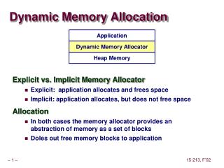
Background • Allocate memory to parallel processors • Goals: • Each processor has sufficient memory • Not too much memory is wasted
Background • Problem: memory requirement may vary over time • If each processor can access only one memory, this is inefficient • If all processors share a single memory, there is heavy contention
Suggested model • Chung et al. [SPAA 2004] suggest a new architecture • Each memory may be accessed by at most two processors • This avoids the mentioned problems
Bin packing • They abstract this problem as a bin packing problem • Bins = memories • Items = memory requirements of processors • Thus, items may be larger than 1
Bin packing • Items may be split and distributed among more than one bin • Condition: each bin contains at most two parts of items • Corresponds to: each memory may be accessed by at most two processors • We also consider the model where each bin may contain k parts of items
Bin packing Processor 1 2 3 4 5 Requirement Assignment 1,2 3,4 2 3,4,5 1 Bins
Notes • There may be many bins which are not full • An item may be split more than once • No upper bound on how often each item is split
Results • Chung et al. [SPAA 2004]: • (k=2) NP-hardness • (k=2) 3/2-approximation • Epstein & vS [WADS 2007]: • (k=2) 7/5-approximation • For general k: • Next Fit is (2-1/k)-approximation • NP-hardness in the strong sense
Results Epstein & vS [WAOA 2007]: • A polynomial time approximation scheme (PTAS) for every (constant) k • For every constant >0, a polynomial time algorithm that uses at most 1+ times the minimal number of bins • at most OPT additional bins of size 1
Results Epstein & vS [WAOA 2007]: • A dual approximation scheme for every (constant) k • For every constant >0, a polynomial time algorithm that uses bins of size 1+ • Larger bins, but no additional bins
Next Fit in this context • If current bin contains k parts of items or is fulll, open a new bin • Put as much as possible of the current item in the current bin • Open additional bin(s) if needed (for large items)
Next Fit: lower bound • One item of size Mk-1 • Next Fit uses Mk-1 bins • M (k-1)k very small items • Next Fit puts k items in one bin, uses M (k-1) bins M (k -1) Mk -1
Next Fit: lower bound • Optimal solution needs only Mk bins • Ratio: (M (2k-1)-1) /Mk2 – 1/k M (k -1) Mk -1 Mk
Next Fit: upper bound • Block = set of full bins, followed by a bin with k items • Each bin >1 in a block was opened because the previous one was full
Weights • Weight of item with size s = s/k • There are at least s parts of item with size s in any packing • OPT is at least the total weight of all the items
Next Fit: upper bound • Consider last bin in a block (not the last block) • Has k items, so at least k -1 items of weight 1/k (these items are not split!) • Block has 1 bin, then k such items • Else, consider all items in block except the k -1 last items
Next Fit: upper bound • S = all items in block exceptthe k -1 last items • How many items are in S ? Unknown! • What is the minimal weight of S ? • Weight = , minimized for single item
Next Fit: upper bound • S = all items in block exceptthe k -1 last items • For block of size b, total size of items in S is strictly more than b -1 • Total weight is then at least b /k • Weight in block at least b /k +(k -1)/k • Note: also true for block of size 1
The last block • Only one bin: weight at least 1/k (has at least one item) • b >1 bins: weight at least b /k • Let size of block i be bi , then Next Fit uses bins • We know that OPT is at least the total weight
Next Fit: upper bound • Let m be the amount of blocks • Also, OPT > NF – m (in each block, at most one bin is not completely full)
Next Fit: upper bound Combining this we find
This talk • We only discuss the algorithms for k=2 • General properties • PTAS • Dual PTAS
Representation of solutions • A solution can be seen as a graph • Vertices = items • An edge between two items = Parts of these two items share a bin • A loop means that a bin contains just one part of an item • We can assume a forest (with loops) • Cycles can be easily removed without changing the cost (Chung et al.,2004).
Example Items:
Additional properties • There exists an optimal packing forest where all items of size in (0,1/2] are leaves or singletons • If the forest representation is minimal (no tree can be split) then a packing is implied from the tree • Can be done iteratively • Singletons are packed into separate bins • A leaf is packed with a maximum amount of its neighbor, and removed from the forest
(Different) example 0.4 1.5 0.9 0.2 1 0.3 0.2
0.6 0.8 1 0.4 0.9 0.3 0.1 0.2 Packing process
PTAS for k=2 • We would like to use standard methods such as • Linear grouping and rounding • Enumeration of patterns • But • Patterns are trees • Items sizes are not bounded from above
New tricks • Optimal packing is adapted in order to make it possible to imitate it • Trees are “truncated” • Partitioned into smaller trees • Large items are truncated • Partitioned into several items that are still large, but bounded • The last two adaptations increase the number of bins by a factor of 1+
Trying all trees • Type of a tree is (j,E) • j is number of edges • E is set of j-1 edges (so that it is a tree) • Pattern = type plus vector of length j • Element i in the vector indicates group of node i • Constant number of patterns • Only question: how many of each?
Dual PTAS for k=2 (briefly) • We use an integer parameter K, based on . • Items can be rounded down to a sizes of the form i/K • We round some non-zero sizes into zero! • By scaling, we get items of integer sizes, and a bin size K
Cutting • There is no reason to cut items at non-integer point • For each item size (at most K), we define cutting patterns • We “guess” how to cut the input items • Using enumeration
Finding a solution • We use a layered graph to find an optimal packing for each option • If the cutting was applied, the problem becomes much easier • However, we did not cut items larger than the bin size • We cut a piece off each one of them, but do not decide on all cutting points • The best (smallest number of bins) option is chosen • Increasing items back to original sizes increases bins slightly
Open problems • PTAS, dual PTAS for non-constant k • (FPTAS or dual FPTAS are most likely impossible since the problem is strongly NP-hard for every constant value of k) • Generalize 7/5-approximation for larger k
7/5-approximation • We show an approximation algorithm for k=2 (at most two parts of items per bin allowed) • First it sorts the items • Then it packs them, starting with the most difficult ones: size between ½ and 1 • We use Next Fit as a subroutine
Step 1: Sorting • Items of size at most ½ are small • Sort them in order of increasing size • Items larger than 1 are large • Sort them in order of decreasing size • Other items are medium-sized • Sort them in order of decreasing size • We pack these items first
Step 2: medium-sized items • Pack medium-sized items one by one: • If current item fits in one bin with the smallest unpacked small item, pack them together • Else, pack current item together with two largest unpacked small items in two bins
Step 3: all small items are packed • We do this until we run out of either the medium-sized or the small items • If all small items are packed, use Next Fit on rest, start with medium-sized items
Step 4: some small items remain • Pack each small item in its own bin • Pack large items into these bins using Next Fit • Still use ordering from before: • Largest large items first • Smallest small items first
Step 5: small items left • We have now run out of either the large or the small items • If bins with small items remain, repack these items two per bin
Step 6: large items left • Pack remaining large items using Next Fit
Upper bound • We use the same weight definition as before: weight of item with size s is • We know that OPT is at least the total weight • How much weight do we pack in a bin?
Amount of weight packed Step 2: • Pack medium-sized items one by one: • If current item fits in one bin with the smallest unpacked small item, pack them together. Weight ½+½ = 1 • Else, pack current item together with two largest unpacked small items in two bins. Three items of weight ½ in two bins: ¾
Amount of weight packed Step 3: • If all small items are packed, use Next Fit on rest, start with medium-sized items • We assume many small items exist • Then, this step does not occur
Amount of weight packed Step 4: • Pack each small item in its own bin • Pack large items into these bins using Next Fit • Still use ordering from before: • Largest large items first • Smallest small items first
Amount of weight packed • Consider a large item which is packed into g bins • It is packed together with g small items (total weight g /2) • The large item has size strictly more than (g -1)/2, so weight at least g /4 • Average weight per bin = 3/4
Amount of weight packed Step 5: • We have now run out of either the large or the small items • If bins with small items remain, repack these items two per bin • Weight: ½ + ½ = 1