Helioseismology

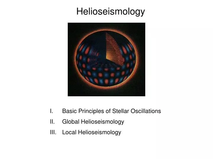
1. Helioseismology • Basic Principles of Stellar Oscillations • Global Helioseismology • Local Helioseismology

2. The birth of helioseismology

3. Take a postive image in a blue-shifted band pass Take a negative image in a red-shifted band pass A Dopplergram Add the two. No velocity is gray, postive, negative velocities appear white/dark

4. A modern Dopplergram from space (SOHO)opplergram

6. where Ylm(q,f) is the associated Legendre function I. Basic Principles of Stellar Oscillations • Notation for Normal Modes of Resonance: • Oscillations within a spherical object can be represented as a superposition • of many normal modes , each which varies sinusoidally in time. The • velocity due to pulsations can thus be expressed as: ∞ ∞ l –imf ∑ ∑ ∑ v(r,q,f,t) = Vn(r) Ylm(q,f)e m=–l n=0 l=0 Vn(r) is the radial part of the velocity displacement n,l, and m are the „quantum“ numbers of the stellar oscillations where: nis the radial quantum number and is the number of radial nodes (order) lis the angular quantum number (degree) mis the azimuthal quantum number

7. The number of nodes intersecting the pole = m The number of nodes parallel to the equator = l– m The angular degree l measures the horizontal component of the wave number: kh = [l(l + 1)]½ /r at radius r

8. Sectoral mode Zonal mode Low degree modes High degree modes

9. Types of Oscillations To get stable oscillations you need a restoring force. In stars oscillations are classified by 3 major modes depending on the nature of the restoring force: p-modes: pressure is the restoring force (example: Cepheid variable stars) g-modes: gravity is the restoring force (example: ocean waves). As we shall see this is also related to the buoyancy force. f-modes: fundamental modes. g- or p-modes that do not have a radial node In the sun p-modes have periods of minutes, g-modes periods of hours

10. Characteristic Frequencies Stellar oscillations are characterized by two frequencies, depending on whether pressure or gravity is the restoring force. Lamb Frequency: The Lamb frequency is the reciprocal time scale defined by the horizontal wavelength divided by the local sound speed: l(l +1)cs2 Ll2 = (khcs)2 = r2 k = 2p/l Travel time t = (1/k)/cs Frequency = 1/t

11. dlnr ) 1 ( dlnP N2 = g – g dr dr Characteristic Frequencies Brunt-Väisälä Frequency The frequency at which a bubble of gas may oscillate vertically with gravity the restoring force: • is the ratio of specific heats = Cv/Cp g is the gravity Where does this come from? Remember the convection criterion?

12. r2 P2 r2* DT Dr P2* Dr P = rg g = CP/CV = 5/3 Cp, Cv = specific heats at constant V, P r1* After the perturbation: r1 P1* P1 P2* 1/g ( ) P2 = P2* r2* = r1 P1* Convection: The Brunt-Väisälä Frequency Consider a parcel of gas that is perturbed upwards. Before the perturbation r1* = r1 and P1* = P1 For adiabatic expansion:

13. Convection: The Brunt-Väisälä Frequency Stability Criterion: Stable: r2* > r2 The parcel is denser than its surroundings and gravity will move it back down. Unstable: r2* < r2 the parcel is less dense than its surroundings and the buoyancy force will cause it to rise higher.

14. 1/g 1/g 1/g r2* ( P2 ) { } { } = = = r1 P1 P1 r1 1 ( dP ) Dr r2* = r1 + g dr P P1 + Dr dr dP r2 = r1 + Dr dr dr Dr 1 + dr 1 dP > P dr dr r1 1 ( dP ) This is the Schwarzschild criterion for stability g dr P Convection: The Brunt-Väisälä Frequency Stability Criterion:

15. r2 P2 r2* DT Dr P2* Difference in density between inside the parcel and outside the parcel: r1 1 Dr ( dP ) Dr r2* = r1 + g dr P dr r2 = r1 + Dr dr – Dr = r1* r1 dlnr 1 ( dlnP ) P1* r r Dr – Dr = dr g dr P1 r 1 ( dP ) Dr dlnr dr ( dlnP ) g 1 dr r P Dr Dr – r Dr = dr dr g dr Convection: The Brunt-Väisälä Frequency

16. dlnr ( dlnP ) 1 A = – g dr dr Buoyancy force: FB = –DrVg V = volume FB = –kx w2 = k/m For a harmonic oscillator: dlnr ( dlnP ) 1 N2 = grAV/Vr = gA = g – g dr dr The Brunt-Väisälä Frequency is the just the harmonic oscillator frequency of a parcel of gas due to buoyancy Dr = rADr FB = –grAVDr In our case x = Dr, k = grAV, m ~ rV

17. Characteristic Frequencies The frequency of the oscillations indicate the type of the restoring force. Ifsis the frequency of the oscillation: s2 > Ll2, N2: For high frequency oscillations the restoring force is mainly pressure and oscillations show the characteristic of acoustic (p) modes. s2 < Ll2, N2: For low frequency oscillations the restoring force is mainly due to buoyancy and the oscillations show the characteristic of gravity waves. Ll2 < s2 < N2, Ll2 > s2 > N2 : In these regions of the star evanescent waves exist, i.e. the wave exponentially decreases with distance from the propagation region.

18. Propagation Diagrams p-modes p-modes Decaying waves g-modes Decaying waves g-modes g modes cannot propagate through the convection zone. Why? Buoyancy force is a destabilizing force. Propagation diagrams can immediately tell you where the p- and g-modes propagate

19. c = √gp/r ) ( ∂lnp g = ∂lnr S Probing the Interior of the Sun: p-modes The period is determined by the travel time of acoustic waves in a cavity defined by two turning points: one just below the photosphere where the where the density decreases rapidly (reflection), and a lower turning point caused by the gradual increase of the sound speed, c, with depth (refraction). At the lower reflection point the wave is traveling horizontally and the reflection occurs at a depth d where c = 2ps/kh

20. Red: high degree modes have shorter wavelengths and do not propagate deeper into the sun. Decreasing density causes the wave to reflect at the surface Increasing density causes the wave to refract in the interior. Blue: low degree modes have longer wavelengths and propagate deeper into the sun.

21. By observing modes with a range of frequencies one can sample the sound speed with depth:

22. Dn0 l=0 l=1 l=2 Assymptotic Relationship for P-mode oscillations (n>> l) p-modes: nnl≈ Dn0 (n + l/2 + e) + dn Tassoul (1980) • is a constant that depends on the stellar structure Dn0 = [2∫0Rdr/c]–1 where c is the speed of sound (i.e. this is the return sound travel time from the surface to the core) dn = small spacing (related to gradient in sound speed) p-modes are equally spaced in frequency n

23. The Small Frequency Spacing

24. A(l + 1)l– h (n + l/2 + e) R (l + 1) dc dr ∫ dn,l = Dn0 dr r 2p2nn,l 0 The Small Frequency Spacing Normally modes of different n and l that differ by say –1 innand +2 inlare degenerate in frequency. In reality since differentlmodes penetrate to different depths this degeneracy is lifted. nn,l= Dn0 (n + l/2 + d) – A,h,e depend on the structure of the star The small separation is sensitive to sound speed gradients

25. Probing the Interior of the Sun: g-modes For g-modes wave propagation is generally only possible in regions of the Sun below the convection zone. A particular g-mode is trapped in regions where its frequency s is less than the local buoyancy frequency N. The upper and lower reflection points of any given cavity correspond to where N has approached s. G-modes thus sample the Brunt-Väisälä frequency, N, as a function of depth The g-modes all share the reflection point near the base of the convection zone and their amplitudes decay throughout that zone (evanescent). Since the decay rate increases withlonly low degree modes are likely to be detected in the atmosphere.

26. Assymptotic Relationship for G-mode oscillations (n>> l) g-modes: n + ½ l + g P0 Pn,l≈ [l(l+ 1)]½ rc –1 dr [ ] ∫ P0 = 2p2 N r 0 P0 g-modes are equally spaced in Period l=0 l=1 l=2 n

27. dlnr ) 1 ( dlnP N2 = g – g dr dr c = √gp/r The basis of Helioseismology P-modes enable you to probe the sound speed with depth. The sound speed is related to the pressure and density, thus you probe the pressure and density with depth. G-modes enable you to probe the Brunt-Vaisaila frequency with depth. This frequency depends on the gravity, and gradient of the pressure and density

28. Excitation of Modes Normally, when a star undergoes oscillations dissipative forces would cause the oscillations to quickly damp out. You thus need a driving force or excitation mechanism to sustain the oscillations. Two possible mechanisms: • Mechanism: • The energy generation depends sensitively on the temperature. If a star contracts the temperature rises and the energy generation increases.This mechanism is only important in the core, and is not an important mechanism in the Sun.

29. Excitation of Modes • Mechanism: • If in a region of the star the opacity changes, then the star can block energy (photons) which can be subsequently released in a later phase of the pulsation. Helium and and Hydrogen ionization zones of the star are normally where this works. Consider the Helium ionization zone in the interior of a star. During a contraction phase of the pulsations the density increases causing He II to recombine. Neutral helium has a higher opacity and blocks photons and thus stores energy. When the star expands the density decreases and neutral helium is ionized by the emerging radiation. The opacity then decreases. • This mechanism is reponsible for the 5 minute oscillations in the Sun.

30. II. Helioseismology The solar 5 min oscillations were first thought to be just convection motion. Later it was established that these were acoustic modes trapped below the photosphere. The sun is expected to have millions of these modes. The amplitude of detected modes can be as small as 0.2 m/s

31. Currently there are several thousands of modes detected withl up to 400. These are largely the result of global networks which remove the 1-day alias. These p-mode amplitude have a Gaussian distribution centered on a frequency of 3 mHz

32. To find all possible pulsaton modes you need continuous coverage. There are three ways to do this. Ground-based networks: Telescopes that are well spaced in longitude. South pole in Summer Spaced-based instruments

33. GONG: Global Oscillation Network Group • Big Bear Solar Observatory: California, USA • Learmonth Solar Observatory: Western Australia • Udaipur Solar Observatory: India • Observatory del Teide: Canary Islands • Cerro Tololo Interamerican Observatory: Chile • Mauno Loa: Hawaii, USA • BiSON: Birmingham Solar Oscillation Network • Carnarvon, Western Australia • Izaqa, Tenerife • Las Campanas, Chile • Mount Wilson, California • Narrabri, New South Wales, Australia • Sutherland, South Africa

34. SOHO: Solar and Heliospheric Observatory is a ESA/NASA project to observe the sun. It is located at the L1 point Three helioseismology experiments: MDI (Michelson-Doppler Imager), GOLF (Global Oscillations Low Frequency) and VIRGO L1 is where gravity of Earth and Sun balance. Satellites can have stable orbits with minimum energy use

35. The p-mode Fourier spectrum from GOLF, using a 690-day time series of calibrated velocity signal, which exhibits an excellent signal to noise ratio.

36. The low-frequency range of the p modes from above spectrum, showing low-n order modes.

38. Rise to low frequency due to stochastic noise of convection

39. Two useful methods of plotting the bewildering number of pulsation modes on the Sun are via „Ridge“ Diagrams and „Echelle“ diagrams Ridge Diagrams are more common in Helioseismology, while Echelle diagrams are more common for Asteroseismology (explained in next lecture).

40. Christensen-Dalsgaard Notes Ridge diagrams plot the amplitudes of solar modes as a function of frequency and degree number. f-mode is the fundamental mode, n=0

41. Ridge Diagrams for the Sun Color symbolizes power

42. Thick line: inversion Thin line model Results from Helioseismology There are two ways of deriving the internal structure of the sun • Direct Modelling • Computationally easy • Results depend on model • Inversion Techniques • Model independent • Computationally difficult

43. Sound Speed: P-modes give information about the sound speed as a function of depth. The sound speeds in the mid-region of the radiative zone were found to be off by 1%. This suggested that the opacity below the convection zone was underestimated. This has since been confirmed by new opacities.

45. Deviations of the sound speed from the solar model red is positive variations (hotter) and blue is negative variations (cooler regions). From SOHI MDI data.

46. Possibly due to increased turbulence Note change of scale from previous graph Deviations of the observed sound speed from the model. The differences are mostly less than 0.2%

47. Simple convection (mixing length theory) does not adequately model observed frequencies Mixing length theory: A hot blob moves a certain distance upwards and deposits all of its excess energy into the surrounding region. It is a flux source. L

48. Rotation: With no rotation allmmodes from a givenlare degenerate. Rotation lifts this degeneracy and them. For anl=1, m = –1,0,+1. Thus rotational splitting will be a triplet. Analogy: Zeeman splitting of energy levels of atom. l = 1 stellar oscillator with modes split into triplets by rotation.

50. Rotation profiles of the Sun‘s interior at 3 latitudes. Note that differential rotation only occurs in the convective core.