Download

1 / 19
280 likes | 909 Views
Effective Gaussian mixture learning for video background subtraction. Dar-Shyang Lee, Member, IEEE. Outline. Introduction Mixture of Gaussian models Adaptive mixture learning Background subtraction Experimental results Conclusions. Introduction. Adaptive Gaussian mixtures:

E N D
Effective Gaussian mixture learning for video background subtraction Dar-Shyang Lee, Member, IEEE
Outline • Introduction • Mixture of Gaussian models • Adaptive mixture learning • Background subtraction • Experimental results • Conclusions
Introduction • Adaptive Gaussian mixtures: • Used for modeling nonstationary temporal distributions of pixels in video surveillance applications for a long time • Been employed in real-time surveillance systems for background subtraction and object tracking • Balancing problem: • Convergence speed and stability • The rate of adaptation is controlled by a global parameter that ranges between 0 and 1. • too small : Slow convergence • too large : Modeling too sensitive
Introduction • This paper proposes an effective online learning algorithm to improve the convergence rate without compromising model stability • Replacing the global, static retention factor with an adaptive learning rate calculated for each Gaussian at every frame • Significant improvements are shown on both synthetic and real video data.
Mixture of Gaussian models • Goal: • Flexible enough to handle variations in lighting, moving scene clutter, multiple moving objects and other arbitrary changes to the observed scene • Modeling each pixel as a mixture of Gaussians and the adaptive mixture model are then evaluated to determine which are most likely to result from a background process. • Our background method contains two significant parameters –α, the learning constant and T, the proportion of the data that should be accounted for by the background.
Mixture of Gaussian models • New frame arrives: • Update parameters of the Gaussians • The Gaussians are evaluated using a simple heuristic to hypothesize which are most likely to be part of the “background process.”
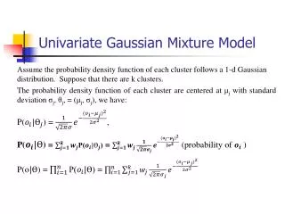
Mixture of Gaussian models • The probability of observing the current pixel value is • Gaussian probability density function • Every new pixel value, Xt, is checked against the existing K Gaussian distributions • A match is defined as a pixel value within 2.5 standard deviations of a distribution1.
Proposed Algorithm • The parameters of the distribution which matches the new observation are updated as follows • Background Model Estimation • Consider the accumulation of supporting evidence and the relatively low variance for the “background” distributions • New object occludes the background object • Increase in the variance of an existing distribution. • First, the Gaussians are ordered by the value of ω/σ.
Background Model Estimation • First, the Gaussians are ordered by the value of ω/σ. • Then, the first B distributions are chosen as the background model • T is a measure of the minimum portion of the data that should be accounted for by the background • Small T: unimodal • Large T: multi-modal
Adaptive mixture learning • Learning rate schedule: • : Local estimate • : Learning rate • A solution that combines fast convergence and temporal adaptability is to use a modified schedule • is computed for each Gaussian independently from the cumulative expected likelihood estimate.
Proposed Algorithm • The basic algorithm follows the formulation by Stauffer and Grimson [9] • Differences: • • • [9] C. Stauffer and W.E.L. Grimson, “Adaptive Background Mixture Models for Real-Time Tracking,” Proc. Conf. Computer Vision and Pattern Recognition, vol. 2, pp. 246-252, June 1999.
Proposed Algorithm • This modification significantly improved the convergence speed and model accuracy with almost no adverse effects. • Winner-take-all option where only a single best-matching component is selected for parameter update is typically used. • Starvation problem • Soft-partition: All Gaussians that match a data point are updated by an amount proportional to their estimated posterior probability • Improve robustness in early learning stage for components whose variances are too large and weights too small to be the best match.
Background subtraction • Temporal distribution P(x) of pixel x • Density estimate • We train a sigmoid function on w/α to approximate P(B|Gk) using logistic regression • The foreground region is composed of pixels where P(B|x) < 0.5.
Experimental results • The proposed mixture learning is tested and compared to conventional methods[9] using both simulation and real video data. • Mixture Learning Experiment • Evaluated through quantitative analysis on a set of synthetic data. • Converged faster and achieved better accuracy. • Background Segmentation Experiment • Successful segmentation in early stage • Quick convergence [9] C. Stauffer and W.E.L. Grimson, “Adaptive Background Mixture Models for Real-Time Tracking,” Proc. Conf. Computer Vision and Pattern Recognition, vol. 2, pp. 246-252, June 1999.
Conclusions • We presented an effective learning algorithm that improved convergence rate and estimation accuracy over the standard method used today • The results were verified by a large number of simulations over a range of parameter settings and distributions.